Free Energies and Variational Inference

My Labor Day Holiday Blog: for those on email, I will add updates, answer questions, and make corrections over the next couple weeks. Thanks for reading and enjoy ! Wubba dub dub.

My graduate advisor used to say:

“If you can’t invent something new, invent your own notation”

Varitional Inference is foundational to Unsupervised and Semi-Supervised Deep Learning. In particular, Variational Auto Encoders (VAEs). There are many, many tutorials and implementations on Variational Inference, which I collect on my YouTube channel and below in the references. In particular, I look at modern ideas coming out of Google Deep Mind.

The thing is, Variational inference comes in 5 or 6 different flavors, and it is a lot of work just to keep all the notation straight.

We can trace the basic idea back to Hinton and Zemel (1994)– to minimize a Helmholtz Free Energy.

What is missing is how Variational Inference is related the Variational Free Energy from statistical physics. Or even how an RBM Free Energy is related to a Variational Free Energy.

This holiday weekend, I hope to review these methods and to clear some of this up. This is a long post filled with math and physics–enjoy !

Generating Functions

Years ago I lived in Boca Raton, Florida to be near my uncle, who was retired and on his last legs. I was working with the famous George White, one of the Dealers of Lightening, from the famous Xerox Parc. One day George stopped by to say hi, and he found me hanging out at the local Wendy’s and reading the book Generating Functionology. It’s a great book. And even more relevant today.

The Free Energy, $\mathcal{F}=ln; Z$ is a Generating function. It generates thermodynamic relations. It generates expected Energies through weight gradients $\nabla_{W}$ . It generates the Kullback-Liebler variational bound, and its corrections, as cumulants. And, simply put, in unsupervised learning, the Free Energy generates data.

Let’s see how it all ties together.

Inference in RBMs

We first review inference in RBMs, which is one of the few Deep Learning examples that is fully expressed with classical Statistical Mechanics.

Suppose we have some (unlabeled) data $\mathbf{x}\in D$ . We know now that we need to learn a good hidden representation ( $\mathbf{v}\rightarrow\mathbf{h}$ ) with an RBM, or, say, latent ( $\mathbf{x}\rightarrow\mathbf{z}$ ) representation with a VAE.

Before we begin, let us try to keep the notation straight. To compare different methods, I need to mix the notation a bit, and may be a little sloppy sometimes. Here, I may interchange the RBM and VAE conventions

$hidden\;(\mathbf{h})\leftrightarrow\;latent\;(\mathbf{z})$

$data\;(\mathbf{x})\leftrightarrow visible\;units\;(\mathbf{v})$

and, WLOG, may interchange the log functions

$ln\;x\leftrightarrow\;log\;x$

and drop the parameters on the distributions

$q, p\leftrightarrow q_{\phi},p_{\theta}\;\;.$

Also, the stat mech Physics Free Energy convention is the negative log Z,

$\mathcal{F}=-\beta\ln\;Z\;\;.$

and I sometimes use the bra-ket notation for expectation values

$\mathbb{E}[x]=\langle x\rangle\;$ .

Finally I might mix up the minus signs in the early draft of this blog; please let me know.

In an RBM, we learn an Energy function $, explicitly:

$E(\mathbf{v},\mathbf{h})=\mathbf{a}^{T}\mathbf{v}+\mathbf{b}^{T}\mathbf{h}+\mathbf{v}^{T}\mathbf{W}\mathbf{h}$

Inference means gradient learning. along the variational parameters $\theta=[\mathbf{a},\mathbf{b}, \mathbf{W}]$ , for the expected log likelihood

$\nabla_{\theta}\mathbb{E}[log\;p(\mathbf{x})]$ .

This is actually a form of Free Energy minimization. Let’s see why…

The joint probability is given by a Boltzmann distribution

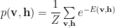
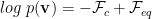
$p(\mathbf{v},\mathbf{h})=\dfrac{1}{Z}\sum \limits_{\mathbf{v},\mathbf{h}}e^{-E(\mathbf{v},\mathbf{h})}$ .

To get $log\;p(x)$ , we have to integrate out the hidden variables

$p(\mathbf{v})=\sum \limits_{\mathbf{h}}p(\mathbf{v},\mathbf{h})=\sum\limits_{\mathbf{h}}\left(\dfrac{1}{Z}e^{-E(\mathbf{v},\mathbf{h})}\right)=\dfrac{1}{Z}\sum\limits_{\mathbf{h}}\left(e^{-E(\mathbf{v},\mathbf{h})}\right)$

$log\;p(\mathbf{v})=\log\;\sum\limits_{\mathbf{h}}e^{-E(\mathbf{v},\mathbf{h})}-\log\;Z$

$log\;p(\mathbf{v})=\log\;\sum\limits_{\mathbf{h}}e^{-E(\mathbf{v},\mathbf{h})}-\log\;\sum\limits_{\mathbf{v},\mathbf{h}}e^{-E(\mathbf{v},\mathbf{h})}$

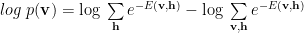
log likelihood = – clamped Free Energy + equilibrium Free Energy

(note the minus sign convention)

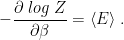
We recognize the second term as the total, or equilibrium, Free Energy from the partition function 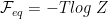$\mathcal{F}_{eq}=-T log\;Z$ . This is just like in Statistical Mechanics (stat mech), but with $T=\dfrac{1}{\beta}=1$ . We call the first term the clamped Free Energy $\mathcal{F}_{c}$ because it is like a Free Energy, but clamped to the data (the visible units). This gives

$log\;p(\mathbf{v})=-\mathcal{F}_{c}+\mathcal{F}_{eq}\;$ .

We see that the partition function Z is not just the normalization–it is a generating function. In statistical thermodynamics, derivatives of $log\;Z$ yield the expected energy

$-\dfrac{\partial\;log\;Z}{\partial\beta}=\langle E\rangle\;.$

Since $T=1$ , we can associate an effective T with the norm of the weights

$T^{eff}\sim\dfrac{1}{\Vert\mathbf{W}\Vert}\;.$

So if we take weight gradients $\nabla_{W_{ij}}$ of the Free Energies, we expect to get something like expected Energies. And this is exactly the result.

The gradients of the clamped Free Energy give an expectation value over the conditional $p(\mathbf{h}|\mathbf{v})$

$\nabla_{\theta}\mathcal{F}_{c}=\mathbb{E}_{p(\mathbf{h}|\mathbf{v})}[\mathbf{h}^{T}\mathbf{v}]\;,$

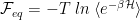
and the equilibrium Free Energy gradient yields an expectation of the joint distribution $p(\mathbf{h},\mathbf{v})$ :

$\nabla_{\theta}\mathcal{F}_{eq}=\mathbb{E}_{p(\mathbf{h},\mathbf{v})}[\mathbf{h}^{T}\mathbf{v}]\;.$

The derivatives do resemble expected Energies, with a unit weight matrix $\mathbf{W}=\mathbf{I}$ , which is also, effectively, $T^{eff}=1$ . See the Appendix for the full derivations.

The clamped Free Energy is easy to evaluate numerically, but the equilibrium distribution is intractable. Hinton’s approach, Contrastive Divergence, takes a point estimate

$\mathbb{E}_{p(\mathbf{h},\mathbf{v})}[\mathbf{h}^{T}\mathbf{v}]\sim\bar{\mathbf{h}}^{T}\bar{\mathbf{v}}\;$ ,

where $\bar{\mathbf{h}}$ and $\bar{\mathbf{v}}$ are taken from one or more iterations of Gibbs Sampling– which is easily performed on the RBM model.

Free Energy Approximations

Unsupervised learning appears to be a problem in statistical mechanics — to evaluate the equilibrium partition function. There are lots of methods here to consider, including

Monte Carlo, which is too hard computationally, and has too high variance
Gibbs sampling + a point estimate, the Hinton CD solution
Variational inference using the Kullback-Leibler bound and the reparameterization trick
Importance, Umbrella sampling, a classic method from computational chemistry
Deterministic fixed point equations, such as the TAP theory behind the EMF-RBM
(Simple) Perturbation theory, yielding a cumulant expansion
and lots of other methods (Laplace approximation, Stochastic Langevin Dynamics, Hamiltonian Dynamics, etc.)

Not to mention the very successful Deep Learning approach, which appears to be to simply guess, and then learn deterministic fixed point equations (i.e. SegNet) , via Convolutional AutoEncoders.

Unsupervised Deep Learning today looks like an advanced graduate curriculum in non-equilibirum statistical mechanics, all coded up in tensorflow.

We would need a year or more of coursework to go through this all, but I will try to impart some flavor as to what is going on here.

Variational AutoEncoders

VAEs are a kind of generative deep learning model–they let us model and generate fake data. There are at least 10 different popular models right now, all easily implemented (see the links) in like tensorflow, keras, and Edward.

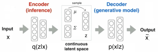
The vanilla VAE, ala Kingma and Welling, is foundational to unsupervised deep learning.

As in an RBM, in a VAE, we seek the joint probability $p(\mathbf{x},\mathbf{z})$ . But we don’t want to evaluate the intractable partition function $Z$ , or the equilibrium Free Energy $F_{eq}=-log\;Z$ , directly. That is, we can not evaluate $\mathbb{E}_{p(\mathbf{x},\mathbf{z})}$ , but perhaps there is some simpler, model distribution $q(\mathbf{z},\mathbf{x})$ which we can sample from.

There are severals starting points although, in the end, we still end up minimizing a Free Energy. Let’s look at a few:

Score matching

This an autoencoder, so we are minimizing a something like a reconstruction error. We need is a score $(\phi)$ between the empirical $p(\mathbf{x})$ and model $q_{\theta}(\mathbf{x})$ distributions, where the partition function cancels out.

$min\;\mathbb{E}_{p(x)}[\;\Vert\phi(p)-\phi(q)\Vert^{2}\;]\;$ .

This is a called score matching (2005). It has been shown to be closely related to auto-encoders.

I bring this up because if we look at supervised Deep Nets, and even unsupervised Nets like convolutional AutoEncoders, they are minimizing some kind of Energy or Free energy, implicitly at $T=1$ , deterministically. There is no partition function–it seems to have just canceled out.

Expected log likelihood

We can also consider just minimizing the expected log likelihood, under the model

$min\;\mathbb{E}_{q}[log\;p(\mathbf{x})]\;$ .

And with some re-arrangements, we can extract out a Helmholtz-like Free Energy. it is presented nicely in the Stanford class on Deep Learning, Lecture 13 on Generative Models.

Raise the Posteriors

We can also start by just minimizing the KL divergence between the posteriors

$min\;KL[q_{\phi}(\mathbf{x}|\mathbf{z})||p_{\theta}(\mathbf{x}|\mathbf{z})]$

although we don’t actually minimize this KL divergence directly.

In fact, there is a great paper / video on Sequential VAEs which asks–are we trying to make q model p, or p model q ? The authors note that a good VAE, like a good RBM, should not just generate good data, but should also give a good latent representation $\mathbf{z}$ . And the reason VAEs generate fuzzy data is because we over optimize recovering the exact spatial information $p(\mathbf{x}|\mathbf{z})$ and don’t try hard enough to get $p(\mathbf{z})$ right.

Variational Bayes

The most important paper in the field today is by Kigma and Welling,where they lay out the basics of VAEs. The video presentation is excellent also.

We form a continuous, Variational Lower Bound, which is a negative Free Energy ( $-\mathcal{L}$ )

$ln\;p(\mathbf{x})=\mathcal{L}_{q(\mathbf{z}|\mathbf{x})}(\mathbf{x})-KL[q_{\phi}(\mathbf{x}|\mathbf{z})||p_{\theta}(\mathbf{x}|\mathbf{z})]$

And either minimizing the divergence of the posteriors, or maximizing the marginal likelihood, we end up minimizing a (negative) Variational Helmholtz Free Energy:

$-\mathcal{L}(\mathbf{x})=\mathbb{E}_{q_{\phi}(\mathbf{z}|\mathbf{x})}[log\;p_{\theta}(\mathbf{z},\mathbf{x}))-log\;q_{\phi}(\mathbf{z}|\mathbf{x})]$

Free Energy = Expected Energy – Entropy

The Kullback-Leibler Variational Bound

There are numerous derivations of the bound, including the Stanford class and the original lecture by Kingma. The take-away-is

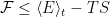
Maximizing the Variational Lower Bound minimizes the Free Energy

The Gibbs-Bogoliubov-Feymnann relation

This is, again, actually an old idea from statistical mechanics, traced back to Feynman’s book (available in Hardback on Amazon for $1300!)

We make it sound fancy by giving it a Russian name, the Gibbs-Bogoliubov relation (described nice here). It is finite Temp generalization of the Rayleigh-Ritz theorem for the more familiar Hamiltonians $\mathcal{H}$ and Hermitian matrices.

The idea is to approximate the (Helmholtz) Free Energy with guess, model, or trial Free Energy $\mathcal{F}_{t}$ , defined by expectations $\le\langle\rangle_{t}$ such that

$\mathcal{F}\le\langle E\rangle_{t}-TS$

$\mathcal{F}_{t}$ is always greater than than true $\mathcal{F}$ , and as our guess expectation $\le\langle\rangle_{t}$ gets better, our approximation improves.

This is also very physically intuitive and reflects our knowledge of the fluctuation theorems of non-equilibrium stat mech. It says that any small fluctuation away equilibrium will relax back to equilibrium. In fact, this is a classic way to prove the variational bound…

and it introduces the idea of conservation of volume in phase space (i.e. the Liouville equation), which, I believe, is related to an Normalizing Flows for VAEs.But that is a future post.

Stochastic Gradients for VAEs

Stochastic gradient descent for VAEs is a deep subject; it is described in detail here

The gradient descent problem is to find the Free Energy gradient in the generative and variational parameters $\nabla_{\phi,\theta}\mathcal{L}(\phi,\theta)$ . The trick, however, is to specify the problem so we can bring variational gradient $\nabla_{\phi}$ inside the expectation value

$\nabla_{\phi}\mathcal{L}()=\mathbb{E}_{q_{\phi}(\mathbf{z}|\mathbf{x})}[\nabla_{\phi}(\cdots)]$

This is not trivial since the expected value depends on the variational parameters. For the simple Free Energy objective above, we can show that

$\nabla_{\phi}\mathcal{L}(\phi)=\mathbb{E}_{q_{\phi}(\mathbf{z}|\mathbf{x})}[(\nabla_{\phi}\;log\;q_{\phi}(\mathbf{z}|\mathbf{x})(log\;p_{\theta}(\mathbf{x},\mathbf{z})-log\;q_{\phi}(\mathbf{z}|\mathbf{x}))]$

Although we will make even further approximations to get working code.

We would like to apply BackProp to the variational lower bound; writing it in these 2 terms make this possible. We can evaluate the first term, the reconstruction error, using mini-batch SGD sampling, whereas the KL regularizer term is evaluated analytically.

We specify a tractable distribution $q(\mathbf{x},\mathbf{z})$ , where we can numerically sample the posterior to get the latent variables $\mathbf{z}\sim q(\mathbf{z}|\mathbf{x})$ using either a point estimate on 1 instance $(\mathbf{x}^{i})$ , or a mini-batch estimate $[\mathbf{x}^{l}|l\in\L$ .

As in statistical physics, we do what we can, and take a mean field approximation. We then apply the reparameterization trick to let us apply BackProp. I review this briefly in the Appendix.

Statistical Physics and Variational Free Energies

This leads to several questions which I will adresss in this blog:

How is this Free Energy related to log Z ?
When is it variational ? When is it not ?
How can it be systematically improved ?
What is the relation to a deterministic, convolutional AutoEncoder ?

Like in Deep Learning, In almost all problems in statistical mechanics, we don’t know the actual Energy function, or Hamiltonian, $\mathcal{H}$ . So we can’t form the instead of Partition Function $\mathcal{Z}$ , and we can’t solve for the true Free Energy $\mathcal{F}$ . So, instead, we solve what we can.

The Energy Representation

For a VAE, instead of trying to find the joint distribution $log\;p(\mathbf{x},\mathbf{z})$ , as in an RBM, we want the associated Energy function, also called a Hamiltonian $\mathcal{H}=E(\mathbf{x},\mathbf{z})$ . The unknown VAE Energy is presumably more complicated than a simple RBM quadratic function, so instead of learning it flat out, we start by guessing some simpler Energy function $\mathcal{H}_{q}=E(\mathbf{z},\mathbf{x})$ . More importantly,We want to avoid computing the equilibrium partition function. The key is, $\mathcal{H}_{q}$ is something we know — something tractable.

And, as in physics, q will also be a mean field approximation— but we don’t need that here.

Perturbation Theory

We decompose the total Hamiltonian into a model Hamiltonian Energy plus perturbation

$\mathcal{H}(\mathbf{x},\mathbf{z})=\mathcal{H}_{q}(\mathbf{x},\mathbf{z})+\lambda\mathcal{V}(\mathbf{x},\mathbf{z})$

Energy = Model + Perturbation

The perturbation is the difference between the true and model Energy functions, and assumed to be small in some sense. That is, we expect our initial guess to be pretty good already. Whatever that means. We have

$\mathcal{V}(\mathbf{x},\mathbf{z})=\mathcal{H}(\mathbf{x},\mathbf{z})-\mathcal{H}_{q}(\mathbf{x},\mathbf{z})$

The constant $latex \lambda\le1&bg=ffffff$ is used to formally construct a power series (cumulant expansion); it is set to 1 at the end.

Write the equilibrium Free Energy in terms of the total Hamiltonian Energy function

$\mathcal{F}_{eq}= -T\;ln\;\langle e^{-\beta\mathcal{H}}\rangle$

There are numerous expressions for the Free Energy–see the Appendix. From above, we have

$\mathcal{F}_{eq}=-ln\;\sum\limits_{\mathbf{x},\mathbf{z}}e^{-\mathcal{H(\mathbf{x},\mathbf{z})}}$

and we define equilibrium averages as

$\mathbb{E}_{eq}[f(\mathbf{x},\mathbf{z})]=\dfrac{1}{Z}\sum\limits_{\mathbf{x},\mathbf{z}}f(\mathbf{x},\mathbf{z})e^{-\mathcal{H(\mathbf{x},\mathbf{z})}}$

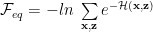
Recall we can not evaluate equilibrium averages, but we can presumably evaluate model averages $\mathbb{E}_{q}[]$ . Given

$\mathcal{H}=\mathcal{H}_{q}+\lambda\mathcal{V}$ ,

where $\lambda\le 1$ , and dropping the $\mathbf{x},\mathbf{z})$ indices, to write

$\mathcal{F}_{eq}= -ln\;[\sum e^{\mathcal{H}_{q}-\lambda\mathcal{V}}]\;.$

Insert $\dfrac{Z_{q}}{Z{q}}=1$ inside the log, where $Z_{q}=\sum e^{-\mathcal{H}_{q}}\;,$ giving

$\mathcal{F}_{eq}= -ln\;[\dfrac{\sum e^{-\mathcal{H}_{q}}}{\sum e^{-\mathcal{H}_{q}}}\sum e^{\mathcal{H}_{q}-\lambda\mathcal{V}}]\;.$

Using the property $ln(xy)=ln(x)+ln(y)$ , and the definition of $\mathbb{E}_{q}$ , we have expressed the Free Energy as an expectations in q.

$\mathcal{F}_{eq}= -ln\;[\sum e^{-\mathcal{H}_{q}}]-ln\;\mathbb{E}_{q}[e^{-\mathcal{V}}]$

This is formally exact–but hard to evaluate even with a tractable model.

We can approximate $ln\;\mathbb{E}_{q}[e^{-\mathcal{V}}]$ with using a cumulant expansion, giving us both the Kullback-Leibler Variational Free Energy, and corrections giving a Perturbation Theory for Variational Inference.

Cumulant Expansion

Cumulants can be defined most simply by a power series of the Cumulant generating function

$ln\;\mathbb{E}[e^{tx}]=t\mu+\dfrac{t^{2}}{2}\sigma^{2}+\cdots$

although it can be defined and applied more generally, and is a very powerful modeling tool.

As I warned you, I will use the bra-ket notation for expectations here, and switch to natural log

$ln\;\mathbb{E}[e^{tx}]=ln\;\langle e^{tx}\rangle$

We immediately see that

the stat mech Free Energy has the form of a Cumulant generating function.

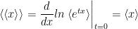
Being a generating function, the cumulants are generated by taking derivatives (as in this video), and expressed using double bra-ket notation.

The first cumulant is just the mean expected value

$\langle\langle x\rangle\rangle=\dfrac{d}{dx}ln\;\langle e^{tx}\rangle\bigg\rvert_{t=0}=\langle x\rangle$

whereas the second cumulant is the variance–the “mean of square minus square of mean”

$\langle\langle x^{2}\rangle\rangle=\dfrac{d^{2}}{dx^{2}}ln\;\langle e^{tx}\rangle\bigg\rvert_{t=0}=\langle x^{2}\rangle-\langle x\rangle^{2}$

(yup, cumulants are so common in physics that they have their own bra-ket notation)

This a classic perturbative approximation. It is a weak-coupling expansion for the equilibrium Free Energy, appropriate for small $V$ , and/or high Temperature. Since we always, naively, assume $T=1$ , it is seemingly applicable when the $q(x,z)$ distribution is a good guess for $p(x,z)$

Kullback Leibler Free Energy and corrections

Since log expectation $ln\;\mathbb{E}_{q}[e^{-\lambda\mathcal{V}}]$ is a cumulant generating function; we can express the equilibrium Free Energy in a power series, or cumulants, in the perturbation V

$\mathcal{F}_{eq}=-ln\;Z_{q}+\lambda\mathbb{E}_{q}[\mathcal{V}]-\dfrac{\lambda^{2}}{2}\mathbb{E}_{q}[\mathcal{V}-\mathbb{E}_{q}[\mathcal{V}]]^{2}+\cdots$

Setting $\lambda=1$ , the first order terms combine with log Z to form the model Helmholtz, or Kullback Leibler, Free Energy

$\mathcal{F}_{q}=-ln\;Z_{q}+\lambda\mathbb{E}_{q}[\mathcal{V}]$

The total equilibrium Free Energy is expressed as the model Free Energy plus perturbative corrections.

$\mathcal{F}_{eq}=\mathcal{F}_{q}+higher\;order\;corrections$

And now, for some

Final Comments and Summary

We now see the connection between the RBMs and VAEs, or, rather between the statistical physics formulation, with Energy and Partition functions, and the Bayesian probability formulation of VAEs.

Statistical mechanics has a very long history, over 100 years old, and there are many techniques now being lifted or rediscovered in Deep Learning, and then combined with new ideas. The post introduces the ideas being used today at Deep Mind, with some perspective from their origins, and some discussion about their utility and effectiveness brought from having seen and used these techniques in different contexts in theoretical chemistry and physics.

Cumulants vs TAP Theory

Of course, cumulants are not the only statistical physics tool. There are other Free Energy approximations, such as the TAP theory we used in the deterministic EMF-RBM.

Both the cumulant expansion and TAP theory are classic methods from non-equilibrium statistical physics. Neither is convex. Neither is exact. In fact, it is unclear if these expansions even converge, although they may be asymptotically convergent. The cumulants are very old, and applicable to general distributions. TAP theory is specific to spin glass theory, and can be applied to neural networks with some modifications.

Perturbation Theory vs Variational Inference

The cumulants play a critical role in statistical physics and quantum chemistry because they provide a size-extensive approximation. That is, in the limit of a very large deep net ( $N\rightarrow\infty$ ), the Energy function we learn scales linearly in N.

For example, mean field theories obey this scaling. Variational theories generally do not obey this scaling when they include correlations, but perturbative methods do.

Spin Glasses and Bayes Optimal Inference

The variational theorem is easily proven using jensen’s inequality, as in David Beli’s notes.

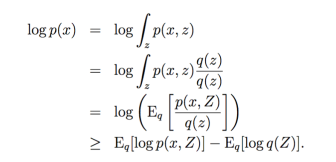
Screen Shot 2017-09-11 at 12.47.08 PM.png

In the context of spin glass theory, for those who remember this old stuff, this means that we have expressions like

$log\;\mathbb{E}[\cdots]_{q}=\mathbb{E}_{q}[log\;(\cdots)]$

which, for a given spin glass model, occurs at the boundary (i.e. the Nishimori line) of the spin glass phase. I will discuss this more in an further post.

Well, it has been a long post, which seems appropriate for Labor Day.

But there is more, in the

Appendix

Derivation of the RBM Free Energy derivatives

I will try to finish this soon; the derivation is found in Ali Ghodsi, Lec [7], Deep Learning , Restricted Boltzmann Machines (RBMs)

VAEs in Keras

I think it is easier to understand the Kigma and Welling paper AutoEncoding Variational Bayes by looking at the equations next to Keras Blog and code. We are minimizing the Variational Free Energy, but reformulate it using the mean field approximation and the reparameterization trick.

The mean field approximation

We choose a model Q that factorizes into Gaussians

$Q(\mathbf{x})=\prod\limits_{i=1}^{N}q_{\phi^{i}}(x_{i})$

$q_{\phi^{i}}(x_{i})=\mathcal{N}(\mu^{i},(\sigma^{i})^{2})$

We can also use other distributions, such as

Being mean field, the VAE model Energy function $mathcal{H}_{q}(\mathbf{x},\mathbf{z})&bg=ffffff$ is effectively an RBM-like quadratic Energy function $E(\mathbf{v},\mathbf{h})$ , although we don’t specify it explicitly. On the other hand, the true $mathcal{H}(\mathbf{x},\mathbf{z})&bg=ffffff$ is presumably more complicated.

We use a factored distribution to reexpress the KL regularizer using

the re-parameterization trick

We can not backpropagate through a literal stochastic node z because we can not form the gradient. So we just replace the innermost hidden layer with a continuous latent space, and form z by sampling from this.

We reparameterize z with explicit random values $\epsilon$ , sampled from a Normal distribution N(0,I)

$\mathbf{z}^{i,,l}=\mathbf{\mu}^{i}+\mathbf{\sigma}^{i}\odot\mathbf{\epsilon}^{l}\;\;\mathbf{\epsilon}^{l}\sim N(0,\mathbf{I})$

Show me the code

In Keras, we define z with a (Lambda) sampling function, eval’d on each batch step

and use this z in the last decoder hidden layer

Of course, this slows down execution since we have to call K.random_normal on every SGD batch.

We estimate mean and variance for the $\mathbf{x}^{i,l}$ in the mini-batch $(l\in L)$ , and sample $\mathbf{z}^{i,l}$ from these vectors. The KL regularizer can then be expressed analytically as

$D_{KL}=\dfrac{1}{2}\sum\limits_{i=1}^{N}1+log(\sigma_{i}^{2}(\mathbf{x}))-\mu_{i}^{2(\mathbf{x})}-\sigma_{i}^{2}(\mathbf{x})$

This is inserted directly into the VAE Loss function. For each a minibatch (of size L), L is

where the KL Divergence (kl_loss) is approximated in terms of the mini-batch estimates for the mean $\mu^{(i)}_{j}$ and variance $\sigma^{(i)}_{j}$ .

in Keras, the loss looks like:

We can now apply BackProp using SGD, RMSProp, etc. to minimize the VAE Loss, with $N(0,\mathbf{I})\rightarrow\mathbf{z}$ on every mini-batch step.

Different expressions for the Free Energy

In machine learning, we use expected value notation, such as

$-\mathcal{F}_{eq}=log\;Z_{eq}=log\;\mathbb{E}_{p((\mathbf{x},\mathbf{z})}[exp[E(\mathbf{x},\mathbf{z})]]$

but in physics and chemistry there at 5 or 6 other notations. I jotted them down here for my own sanity.

For RBMs and other discrete objects, we have

$-\beta\mathcal{F}=ln\sum\limits_{k=0}^{N}exp[-\beta E_{k}]$

Of course, we may want the limit $N\rightarrow\infty$ , but we have to be careful how we take this limit. Still, we may write

$-\beta\mathcal{F}=ln\sum\limits_{k=0}^{\infty}exp[-\beta E_{k}]$

In the continuous case, we specify a density of states $latex \rho(E)&bg=ffffff $

$-\beta\mathcal{F}=ln\int\limits_{0}^{\infty}d\rho(E)exp[-\beta E]$

which is not the same as specifying a distribution $p(\mathbf{x})$ over the internal variables, giving

$-\beta\mathcal{F}=ln\int\limits_{0}^{\infty}d\mathbf{x}p(\mathbf{x})\;exp[-\beta E(\mathbf{x})]$

In quantum statistical mechanics, we replace the Energy with the Hamiltonian operator, and replace the expectation value with the Trace operation

$-\beta\mathcal{F}=ln\;Tr[\;exp[-\beta\mathcal{H}]]$

and this is also expressed using a bra-ket notation

$-\beta\mathcal{F}=ln\langle exp[-\beta\mathcal{H}]\rangle$

and usually use subscripts to represent non-equilibrium states

$-\beta\mathcal{F}_{0}=ln\;Tr[\;exp[-\beta\mathcal{H}_{0}]]$

$-\beta\mathcal{F}_{0}=ln\langle exp[-\beta\mathcal{H}(\mathbf{x})]\rangle_{0}$

Raise the Posteriors

21 Comments

Craig Oknin says:

September 6, 2017 at 12:11 pm

I’m curious – what does knowing the relation of free-energy to deep learning teach us? Does it teach us something about local minima? Does it teach us ways to improve existing algorithms? Does it teach us ways to invent new algorithms? Does it teach us anything about how the mind might work? Does it suggest any new applications?
Thanks.

LikeLike

1. Charles H Martin, PhD says:
  
  September 6, 2017 at 2:07 pm
  
  Current VAEs are not very good. Better methods are needed. Cumulants are a natural way to correct this.
  Of course, cumulants are not the only statistical physics tool. There are other Free Energy approximations, such as the TAP theory we used in the deterministic EMF-RBM.
  
  LikeLike
  
2. Charles H Martin, PhD says:
  
  September 6, 2017 at 2:58 pm
  
  As for the problem of local min–this has been treated with TAP theory nearly 20 years ago. This is the basis of later work by LeCun on spin glasses.
  But really…
  
  It has been known for a long time that these kinds of systems do not suffer from the problems of local minima arise in other optimization provblems. In particular, see the Orange Book on Pattern Recognition and the chapter on neural nets
  
  https://books.google.com/books/about/Pattern_classification.html?id=YoxQAAAAMAAJ
  
  LikeLike
  
  1. Mathieu Blondel says:
    
    September 30, 2017 at 10:35 am
    
    Hi,
    You might be interested in checking out this ICML’17 paper: https://arxiv.org/pdf/1704.08045.pdf
    They have a very concise proof for the fact that most of critical points are global minimum for a class of deep neuron networks with a standard architecture.
    
    LikeLike
    
    1. Charles H Martin, PhD says:
      
      September 30, 2017 at 10:42 am
      
      This proof was started in spin glass theory over 20 years ago
      
      LikeLike
      
    2. Charles H Martin, PhD says:
      
      September 30, 2017 at 10:45 am
      
      And thanks
      
      LikeLike
      
Charles H Martin, PhD says:

September 6, 2017 at 2:11 pm

Beyond that I don’t think a simple cumulants would do better than say applying a skip connection to deal with non local correlations. Hover, for black box variational inference , we need better methods than just vanilla free energy minimization.

LikeLike

Pingback: Distilled News | Data Analytics & R
DJR says:

September 10, 2017 at 10:08 am

Hi, nice post!
I have a similar discussion in my blog: https://danilorezende.com/2015/12/24/approximating-free-energies/

Small observation: While vanilla VAEs are somewhat poor generative models (this is by construction, as they have a simple posterior approximator), Recurrent/Structured VAEs (e.g. (conv)DRAW) aren’t. Recurrent VAEs are as good as PixelCNN/RNVP and are amongst the state-of-the-art in generative models for which there is a standardised evaluation metric.

Let me know if you have any comments,
Cheers

LikeLike

1. Charles H Martin, PhD says:
  
  September 10, 2017 at 10:10 am
  
  Great observation thanks !
  
  LikeLike
  
  1. Charles H Martin, PhD says:
    
    September 10, 2017 at 10:26 am
    
    I would add that even structured variational inference can benefit from tuning. Such as using reinforcement learning to repair the problems and / or to specify structure that is not easy to represent in an RNM .
    
    LikeLike
    
2. Charles H Martin, PhD says:
  
  September 10, 2017 at 11:33 am
  
  Your blog is quite nice, thanks for sharing.
  
  LikeLike
  
Gervase says:

October 11, 2017 at 8:20 am

Working in engineering, I am finding your blog a bit different from my normal reading. But a fascinating subject and one I am determined to understand

LikeLike

1. Charles H Martin, PhD says:
  
  October 12, 2017 at 12:16 pm
  
  The blog is mostly physics oriented. Feel free to ask questions
  
  LikeLike
  
orcera says:

September 8, 2018 at 6:24 am

Thanks for sharing your ideas. Unfortunately, the link to sequential VAEs is broken and thus, I cannot find the paper for your statement: “[…] are we trying to make q model p, or p model q ?”. Can you fix this or give a link to the paper?

LikeLike

1. Charles H Martin, PhD says:
  
  September 8, 2018 at 7:13 am
  
  I guess this got stale. I’ll have to review this post and find some more recent references thanks. On “q model p…” these are my observations..
  
  LikeLike
  
  1. orcera says:
    
    September 8, 2018 at 9:10 am
    
    Thanks for your effort. Would be eager to read about their findings. Thanks!
    
    LikeLike
    
2. Rachel Prudden says:
  
  February 22, 2019 at 8:58 am
  
  It seems the link is still broken. Would be great if anyone could find or guess the relevant paper!
  
  LikeLiked by 1 person
  
  1. Charles H Martin, PhD says:
    
    February 22, 2019 at 9:00 am
    
    LikeLiked by 1 person
    
  2. Charles H Martin, PhD says:
    
    February 22, 2019 at 9:01 am
    
    Sorry IDK what happened to it…seems to be blocked…when i search on youtube I get the Stanford video
    
    LikeLike
    
    1. Rachel Prudden says:
      
      February 22, 2019 at 9:04 am
      
      Oh, how strange. Thanks anyway for the great blog post!
      
      LikeLiked by 1 person

Free Energies and Variational Inference

Generating Functions

Inference in RBMs

Free Energy Approximations

Variational AutoEncoders

Score matching

Expected log likelihood

Raise the Posteriors

Variational Bayes

The Kullback-Leibler Variational Bound

The Gibbs-Bogoliubov-Feymnann relation

Stochastic Gradients for VAEs

Statistical Physics and Variational Free Energies

The Energy Representation

Perturbation Theory

Cumulant Expansion

Kullback Leibler Free Energy and corrections

Final Comments and Summary

Cumulants vs TAP Theory

Perturbation Theory vs Variational Inference

Spin Glasses and Bayes Optimal Inference

Appendix

Derivation of the RBM Free Energy derivatives

VAEs in Keras

The mean field approximation

the re-parameterization trick

Show me the code

Different expressions for the Free Energy

Published by Charles H Martin, PhD

21 Comments

Leave a Reply to Charles H Martin, PhD Cancel reply

Generating Functions

Inference in RBMs

Free Energy Approximations

Variational AutoEncoders

Score matching

Expected log likelihood

Raise the Posteriors

Variational Bayes

The Kullback-Leibler Variational Bound

The Gibbs-Bogoliubov-Feymnann relation

Stochastic Gradients for VAEs

Statistical Physics and Variational Free Energies

The Energy Representation

Perturbation Theory

Cumulant Expansion

Kullback Leibler Free Energy and corrections

Final Comments and Summary

Cumulants vs TAP Theory

Perturbation Theory vs Variational Inference

Spin Glasses and Bayes Optimal Inference

Appendix

Derivation of the RBM Free Energy derivatives

VAEs in Keras

The mean field approximation

the re-parameterization trick

Show me the code

Different expressions for the Free Energy

Share this:

Like this:

Related

Published by Charles H Martin, PhD

21 Comments

Leave a Reply to Charles H Martin, PhD Cancel reply