Describing Double Descent with WeightWatcher

Double Descent (DD) is something that has surprised statisticians, computer scientists, and deep learning practitioners–but it was known in the physics literature in the 80s: And while DD can seem complicated in deep learning models, the original model is actually very easy to understand — and reproduce — with just a few lines of python.

IMHO, DD is a great way to understand how and when Deep Neural Networks might overfit their data, and, moreover, where they achieve optimal performance. And you can do this and more with the open-source weightwatcher tool

https://weightwatcher.ai

The original 1989 DD physics experiment

The original DD experiment from 1989 is easy to set up and run using modern python.

Here’s a notebook that you can run on Google Colab to reproduce all these results, and with a lot more details. (a lot)

One simply trains a Linear Regression to predict the labels of a dataset with binary labels.

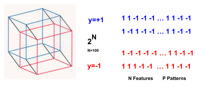
In this case, the data instances are drawn from the vertices of an N-dimensional hypercube and the labels are +1 or -1, depending on the sum of the ‘1s’ in the instance data vector.

This gives the linear equation

where each data vector (x), label (y=[-1|1]), and weight vector (w). Of course, the goal is to learn the N-dimension weight vector (w) given P training data instances.

We can generate the data vectors (x) and their labels (y) using this code (from the notebook):

def generate_mdp_dataset_numpy(P, N):
    X = np.random.choice([-1, 1], size=(P, N))
    Y = generate_majority_labels(X)
    return X, Y

Lets run the experiment 100 times and plot the aveage results. Lets pick features, and let patterns, where is called the load. We vary and compute the test accurary (measured on some random sample).

To just get the resuilts, we can use the scikit-learn LinearRegression module. Again, we run Linear (not Logistic) Regression to predict the binary labels . Here’s the notebook code we use for this.

def run_LR_experiment(alpha=1.0, verbose=True, N=100):

  P = int(alpha * N)

  X_train, Y_train = generate_mdp_dataset_numpy(P,N)
  X_test, Y_test = generate_mdp_dataset_numpy(P,N)

  # Train the linear regression model
  regressor =  LinearRegression(fit_intercept=False)
  regressor.fit(X_train, Y_train)

  # Predict Y values for the training and test sets
  Y_train_value = regressor.predict(X_train)
  Y_test_value  =  regressor.predict(X_test)

  # Convert predictions to binary class labels based on the condition
  Y_train_pred = np.where(Y_train_value > 0, 1, -1)  # Converts to 1 if Y > 0 else -1
  Y_test_pred = np.where(Y_test_value > 0, 1, -1)  # Converts to 1 if Y > 0 else -1


  # Compute accuracy for both training and test sets
  train_accuracy = accuracy_score(Y_train, Y_train_pred)
  test_accuracy = accuracy_score(Y_test, Y_test_pred)

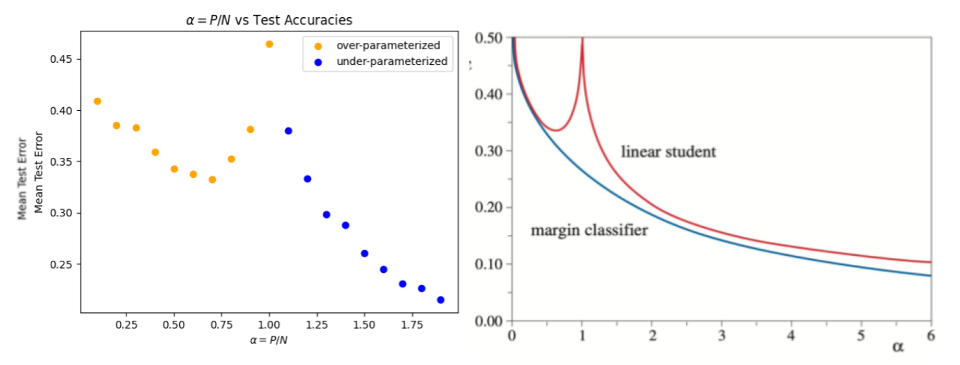
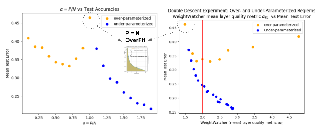
Doing this, we can reproduce the the original DD curve. On the LHS, I reproduced the experiment from the 1989 paper that discovered it . On the RHS, I present theoretical curves (from Opper 1995; ask me for a copy) using both statistical mechanics (StatMech, red) and statistical learning theory (SLT, blue). Notice that it is the StatMech approach that matches experiment. But we don’t need StatMech to understand this…

• N: Number of features / parameters

• P: Number of training examples (i.e Patterns)

• alpha: the ‘load’ parameter (note: this is not the weightwatcher alpha)

There are 2 regimes of interest”:

• under-parameterized: P > N. We have more training data than features. Here, we can always make the model better by just adding more data. Way more data. That’s easy.

• over-parameterized: N > P: We have more features, and therefore more adjustable weights, than training data. Of course, in this simple model, the test accuracy is no better than say 65%. But it does work. And this is the regime most interesting to LLMs and other Deep Neural Networks.

The over-parameterized regime

When , we call this the overparameterized regime. And this is the most interesting regime for LLMs and other DNNs which have a huge number of parameters. Also, this is where traditional statistics falls down.

The traditional stats approach fails to describe the case , where the test error unexpectedly explodes. But, in fact, this is quite easy to describe — and is even predicted — by the weightwatcher theory.

Moreover, when , the test error is minimized. Of course, it is still pretty high, but that’s OK since, again, we will see that, again, this is quite easy to describe — and is even predicted — by the weightwatcher theory. But first,

The PseudoInverse solution

Given a data pair , we can write Linear Regression problem as (where, here, the target variable is just a binary label )

We want to find the weight vector latex \mathbf{X}$ and the vector of labels . We can now write the Linear Regression problem in matrix form as

,We can write the solutions in terms of the Moore-Penrose PseudoInverse. First, lets flip things around a little

Now, multiply by on both sides of this relation

We now invert the data covariance matrix

We now identify the Moore-Penrose PseudoInverse operator

The optimal weight vector is given by

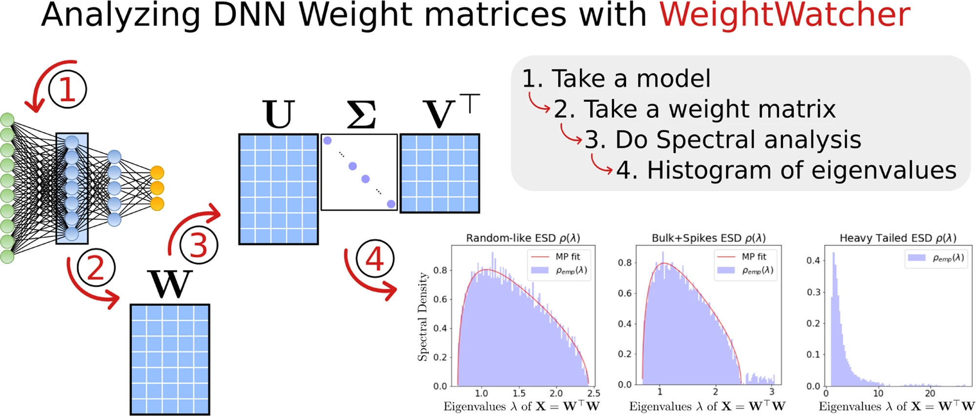
As part of our initial analysis, we will compute the eigenvalues of the  covariance matrix , as described in the paper

as well as the distribution  of the inverse eigenvalues . It is these inverse eigenvalues we will analyze with weightwatcher

The weightwatcher layer quality metric (alpha)

To apply weightwatcher to the PseudoInverse problem, we need to first place the data matrix into a SingleLayerModel (see the notebook), and then use the newly added ‘inverse’ option, which analyzed the inverse covariance matrix of the layer

model = SingleLayerModel(weights=X_train)
watcher = ww.WeightWatcher(model=model)
details = watcher.analyze(inverse=True, plot=True, detX=True)

We can now plot the test accuracy as a function of the weightwatcher layer Power Law (PL) quality metric alpha ). This is shown on the LHS.

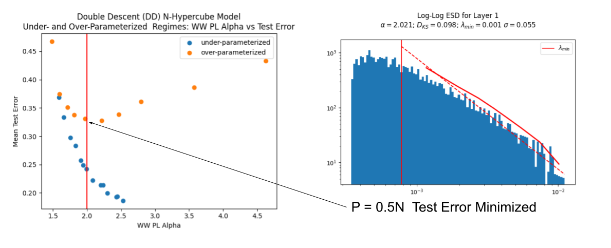
From the left side plot, we immediately see that when

• WW PL-alpha =- 2.0, test error is minimized
• WW-PL-alpha = 1.5. test error is maximized, and the model is severely overfit
• WW PL-alpha > 2.0, test error is sub-optimal as well

Ideal Learning

On the RHS, we drill into the case where , where the test error is minimized. This plot shows the Empirical Spectral Density (ESD) of the (inverse) eigenvalues , and on a log-log scale.

The weightwatcher exactly, which means the ESD can be fit perfectly to a power law distribution with exponent 2.0. This is also exactly where the weightwatcher HTSR theory (as in our JMLR paper) predicts the model would have the best out-of-sample performance!

The WeightWatcher Volume Preserving Transformation

In addition to the Power Law (OK) metric alpha $\alpha_{PL}$, the weightwatcher StatMech theory (discussed in some detail at NeurIPS2023), also states that when the layer is perfectly converged for its data, then the PL tail will form an Effective Correlation Space that satisfies a Volume-Preserving Transformation.

You can check this yourself by adding the detX=True option to the analyze method

details = watcher.analyze(inverse=True, plot=True, detX=True)

and examining the plot on the lower RHS. You can tell your layer is well-trained when the red and purple lines are very close together:

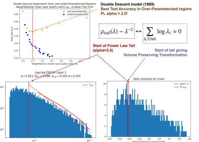
Remarkably, in the case $P=0.5N$, where the test error is minimized, not only is the weightwatcher PL $\alpha_{PL}-2.0$, but the PL tail also satisfies the theoretically predicted volume preserving transformation!

But more importantly, you can use this additional weightwatcher metric to check the quality of your NN layer to see if it is properly converged, or if the layer is is overfit.

Signatures of over-fitting

When the weightwatcher , when , this indicates that the layer ESD is Very Heavy Tailed (VHT), and the underlying weight matrix is atypical. In these case, we can infer that the model is potentially overfit. Again, this is exactly what we see. In other words,

The weightwatcher theory describes the DD curve as predicted

(in the small alpha, overparameterized regime).

Now this is not explained in the old JMLR paper, but I do discuss it at some length in my recent invited talk at NeurIPS2023 (rerecorded). Also see the NeurIPS page for our Workshop on Heavy Tails ML. (with both my original talk and several others)

Why does weightwatcher work so well here. It turns out, for the case , the ESD of the data covariance matrix is the same as the ESD of that Marchenko Pastur random matrix with aspect ratio .

As shown on the LHS below, the ESD has many zero and near-zero eigenvalues $latex \lambda \approx 0$, which was conjectured (back in 1989) to prevent the model from describing out-ot-sample examples.

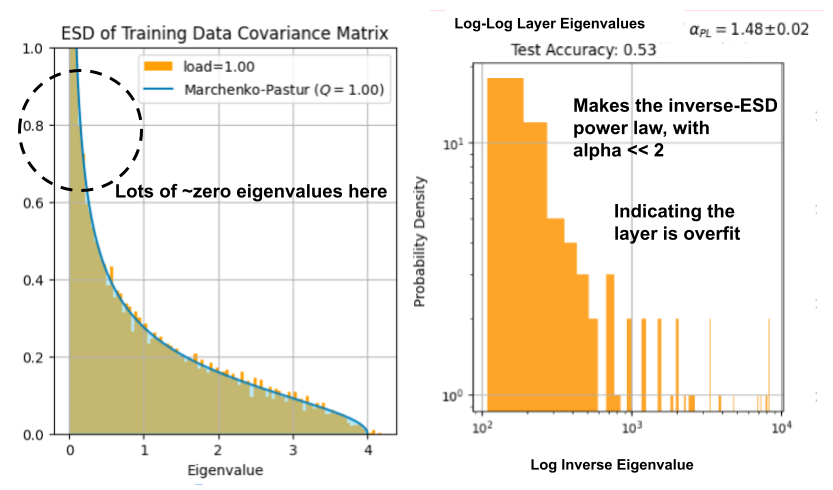
As shown on the RHS (above), when we compute the ESD of the inverse covariance matrix , this ESD can be fit perfectly to a Power Law (PL) distirbution, with alpha exponent $\alpha_{PL}=1.5$ (which is the lower limit of the Clauset esimator weightwatcher users). This means the inverse covariance matrix is highly atypical, and is dominated by the largest (inverse) eigencomponents. Because of this, this matrix is not a typical sample or view on the training data, and it can not describe anything but the training data. In other words, the model is severely overfit.

Also, as shown above, if you add the detX=True option, you can verify that your layer is overfit if the purple line is to the right of the red line. We will discuss this in detail in a future post.

The weightwatcher alpha and the HTSR theory

How are these results related to the basis of weightwatcher–from our JMLR paper on the theory of Heavy Tailed Self-Regularization?

The HTSR theory is a phenomenology that classifies a NN layer weight matrix into a specific Universality Class from Random Matrix Theory (RMT), based on the weightwatcher fit of the Power Law exponent .

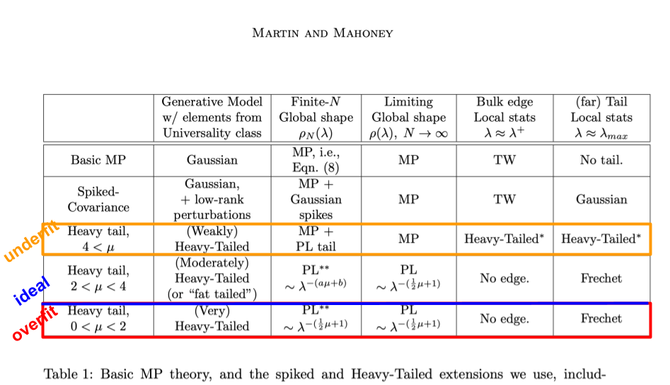
As explained in the paper, when the PL exponent of the ESD is , we can associate the layer with the Heavy-Tailed (HT) Universality Class. When , the HTSR theory predicts that the layer is optimally converged for its training data. And when , the layer ESD is in the Very-Heavy-Tailed (VHT) Universality Class. And as explained in my invited talk at NeurIPS2023, this is a signature that the layer may be overfit, just like in the Double Descent example described here.

Applying weightwatcher to real-world LLMs and DNNs

What can do with weightwatcher ? Ask yourself…

• Do you really know if you using enough data to fine-tune your LLM ?
• Are you worried that you are overfitting the model to your training data
• Are you having trouble evaluating your LLM ?

You can use the tool to find and fix these kinds of problems in your LLMs and NNs that no other tool can diagnose or discover.

WeightWatcher is a one-of-a-kind must-have tool for anyone training, deploying, or monitoring Deep Neural Networks (DNNs).

Learning is an inverse problem. And weightwatcher provides a view into the correlations in the training data, akin to looking at the inverse correlation matrix at different levels of granulairty. And it works even if your data is not random (like this simple model), but correlated, as in a real world problem.

You can use weightwatchet to look for potential signatures of overfitting using the weightwatcher tool. The kind of signatures seen in the classic Double Descent experiment. Even without test data! Even without training data!

You just need to ‘watch’ the model weights.

I developed weightwatcher to help my clients who are training and fine-tuning their own LLMs (and DNN AI models). If it’s useful to you, I’d love to hear about it. And it you need help training or fine-tuning your own models, please reach out. My hashtags are:  #talkToChuck #theAIguy.

In the meantime, remember–Statistical Learning Theory (SLT) cannot describe Double Descent in the over-parameterized regime–but StatMech can. And so can weightwatcher!

Thanks to my friend Patrick Tangphao for this meme (haha)