Deep Learning and Effective Correlation Spaces

AI has taken the world by storm. With recent advances like AlphaFold, Stable Diffusion, and ChatGPT, Deep Neural Networks (DNNs) have had their Sputnik moment. And yet, we really don’t understand why DNNs even work. Unless, of course, you follow this blog and use the widely popular open-source weightwatcher tool.

The open-source weightwatcher tool has been featured in Nature Communications and has over 86K downloads. It can help you diagnose problems in your DNN models, layer-by-layer, without even needing access to the test or training data. But how can weightwatcher possibly do this?

In a previous post, I present the current working theory for the weightwatcher project, which explains where the weightwatcher power law shape metrics alpha $(\alpha)$ , and alpha-hat $(\hat{\alpha})$ really come from. This post has been written up in a new paper, and an early draft available upon request (email me),

I call this SETOL, a SemiEmpirical Theory of Learning.

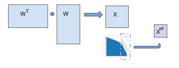
We can write the weightwatcher $(\hat{\alpha})$ metric as an approximate Free Energy/Likeliehood, given as the log model Quality $Q_{T}$ , where the model quality might be the model test accuracy, an average GLUE score, etc. The SETOL approach expresses $Q_{T}$ , in terms of an HCIZ integral

$\mathcal{Q}_{\mathbf{T}}\simeq\log\int d\mu(\mathbf{A})\exp\left(Tr[\mathbf{W}^{T}\mathbf{A}\mathbf{W}]\right),$

It is shown in the SETOL paper that when $\mathbf{W}$ is well trained, the weightwatcher alpha-hat metric is then the approximate log quality

$\hat{\alpha}:=\alpha\log_{10}\lambda^{max}\simeq\log_{10}\mathcal{Q}_{\mathbf{T}},$

In order to formulate this, however, we need to invoke the change of measure $d\mu()$ from the distribution of the full space of all (Student) weight matrices $\mathbf{S}$ to the space of all (Student) correlation matrices,

$d\mu(\mathbf{S})\rightarrow d\mu(\mathbf{A})$

where $\mathbf{A}$ represents an arbitrary ‘Student’ correlation matrix $\mathbf{A}=\frac{1}{N}\mathbf{S}^{T}\mathbf{S}$ .

What does this mean? And, more importantly, how can we be sure it is correct ?

The Effective Correlation Space

First, some more familiar notation. More generally, given an arbitrary layer weight matrix $\mathbf{W}$ , of dimension $N\times M,\;\;N\ge M$ , we define the correlation matrix $\mathbf{X}=\frac{1}{N}\mathbf{W}^{T}\mathbf{W}$ . In this general case, we assume we can perform the change of measure from layer weight matrices $\mathbf{W}$ , to general correlation matrices $\mathbf{X}$ .

$d\mu(\mathbf{W})\rightarrow d\mu(\mathbf{X})$

In words, this means that, we need to change our concept of where the generalizing components live and how we effectively measure them.

For a very well-trained DNN layer, the correlations concentrate into a lower rank space, effectively defined by eigenvalues in the power law (PL) tail of the ESD. By this, we mean that there is some effective operator $\mathbf{X}^{eff}$ that spans the same space as the tail of the ESD (Empirical Spectral Density) . $\rho_{tail}(\lambda)$ and has the same eigenvalues as those eigenvalues $\lambda_{i}$ in the tail of the original layer correlation matrix $\mathbf{X}$ .

This is consistent with the HTSR theory (published in JMLR), that states that for any well-trained weight matrix, the ESD of the layer not only forms a power law $\rho_{tail}(\lambda)\sim\lambda^{-\alpha}$ , but, also, that this tail contains the dominant eigencomponents of $\mathbf{W}$ that allow the model to generalize.

More on what precisely $\mathbf{X}^{eff}$ is in another post; suffice it to say that right now, we just care about the eigenvalues $\lambda$ . And we can test this theory by simply looking at the eigenvalues of our actual weight matrices.

In the rigorous formulation of the weightwatcher theory, to accomplish this, we require that the Effective Correlation Space be defined by a Volume-Preserving Transformation

Volume-Preserving Transformation

if we (crudey) write this transformation in terms of a Jacobian $J(\mathbf{W},\mathbf{X})$ , one can see that to change the measure from the uncorrelated to correlated measure,

$d\mu(\mathbf{W})=J(\mathbf{W},\mathbf{X})d\mu(\mathbf{X})$

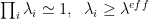
then the Determinant of the Jacobian of this transformation should be the identity, i.e. $\vert J(\mathbf{W},\mathbf{X})\vert=1$ . This can be shown exactly (and is derived in the appendix of the new theory paper)

The key assumption of the weightwatcher theory is an empirically verifiable approximation:

The eigenvalues of the tail of $\lambda_{i}\in \rho_{tail}(\lambda)$ , satisfy the relation $\prod\lambda_{i}=1$ .
That is, the effective correlation matrix $\mathbf{X}^{eff}$ has determinant 1, i.e. $\det \mathbf{X}^{eff}=1$ ,

This means we have now 2 independent methods to identify the power law tail (indicated with a red or purple line.)

MLE fit: (red line): Apply the standard (Clauset MLE) PL estimator, and find the eigenvalue $\lambda_{min}$ where PL the tail starts. This is the default weightwatcher approach.
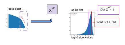
det X=1 (purple line): Search for the first eigenvalue $\lambda^{eff}$ that satisfies condition the $\det \mathbf{X}^{eff}=1$ , condition: $\prod_{i}\lambda_{i}\simeq 1,\;\;\lambda_{i}\ge\lambda^{eff}$

When these 2 methods coincide, we can have great confidence the theory applies well . At least I do.

This constraint can be evaluated empirically by plotting the ESD on a log-linear plot, and comparing the point where to where the PL fit says the tail of the ESD starts (red line) to where the $\det \mathbf{X}^{eff}=1$ constraint is best satisfied (purple line) When these 2 lines overlap, the theory works best. And when they don’t overlap, the layers is not fully optimized.

Remarkably, this is very frequently satisfied when the ESD is power law $\rho_{tail}(\lambda)\sim\lambda^{-\alpha}$ , and has the exponent $\alpha\simeq 2$ , And this, remarkably, according to the HTSR theory, corresponds to optimal learning in that layer!

Empirical Verification of the (SETOL) Theoretical Model

Here, we will provide some justification for these key assumptions, using the open-source weightwatcher tool. As always, all of these results are 100% reproducible, and, moreover, you can test the assumptions on other models yourself.

As always, you can generate these results yourself on any model you like using weightwatcher. Simply use the following commands in your favorite notebook (Jupyter, Google Colab, etc.):

import weightwatcher as ww
watcher = ww.WeightWatcher()
details = watcher.analyze(model=your_model, plot=True, detX=True)

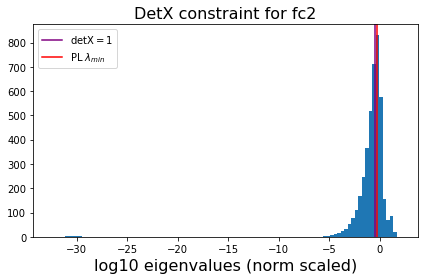
When the theory is working perfectly, or at least as prescribed, then

the weightwatcher Pl shape metric alpha will be about 2: $\alpha\simeq 2.0$
the detX constant plot will show the purple ( $\det \mathbf{X}^{eff}=1$ ) and red ( $x=\lambda_{min}$ ) lines very close together, if not overlapping.

In the theory paper, we show this for a simple example, however, it turns out, this is very common even in many SOTA models!

Here are some examples from SOTA DNN models

ALBERT

ALBERT (A Lite BERT) is a SOTA LLM published by Google & the University of Chicago; it is a lightweight variant of BERT. It even outperforms, BERT, and XLNet, and RoBERTa in some cases.

There are several ALBERT models (base, large, xlarge, xxlarge), and most have layers have $\alpha\in [2.5, 4.5]$ . Here’s a plot of the layer averaged alphas $\langle\alpha\rangle$ for all 4 models, compared their average quality (see this notebook for more details).

Notice that the layer averaged alpha metric, $\langle\alpha\rangle$ , is roughly correlated with model quality. This shows that general weightwatcher approach works on this set of models.

Where the does the SETOL theory work exactly ?

Lets take a look at 2 random layers from. the ALBERT albert-xlarge-v2 model, with different alphas: a middle layer, with $\alpha=2.38$ , and the last layer, with $\alpha=1.83$ . Below you can see that with the smaller alpha of 1.89, closer to 2.0, the purple and red lines overlap.

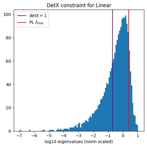
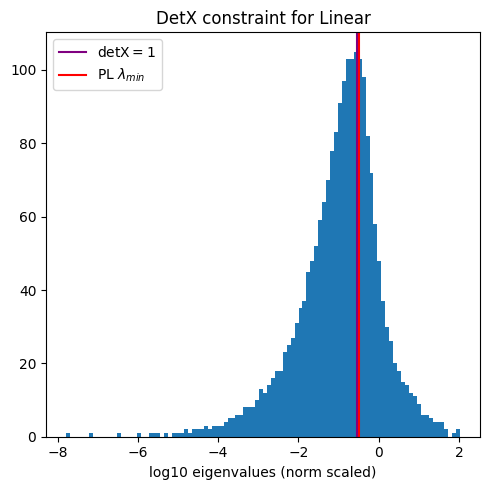
VGG19

We have looked at the VGG series of models before, both in our JMLR paper, and in our Nature Communicationss paper. Here, we look at a couple of Fully Connected (FC) or Dense/Linear layers with alpha near 2.0. (Note, we did this analysis in Table 6, the JMLR paper, but I have found that more recent versions of VGG give different results; here Ireport results from the current, default Keras VGG19 model)

Analysis

Here, despite the 2 plots above looking very different, both alphas are close to 2, and in both cases the purple and red lines overlap, showing that these ESDs exhibit the signatures of the required Volume Preserving Transformation under-the-hood of the rigorous weightwatcher Statistical Mechanics-based Semi-Empirical Theory of Learning (SETOL).

More Models ?

To convince you I am not just cherry-picking examples, let me encourage you to download the open-source weightwatcher tool and try it yourself.

pip install weightwatcher

If you find it works, please let me know. And. if something is wrong, I’d like to know that too.

Closing Points

WeightWatcher is an open-source, diagnostic tool for analyzing Deep Neural Networks (DNN), without needing access to training or even test data. It is based on theoretical research into Why Deep Learning Works, and is described in a new theory–the weightwatcher Semi-Empirical Theory of Learning (SETOL). Here, we have shown a key feature of the new SETOL approach–that DNNs can be described with an Effective Correlation Space at each layer, and that this space is characterized by a Volume Preserving Transformation that captures and concentrates the correlations in the data at each layer. And we have shown how you can test this yourself using the weightwatcher tool.

Most importantly, the empirical results show that when the layer is learning perfectly, the layer correlations can be fit to a heavy-tailed power law (PL) distribution, with PL exponent alpha of 2–exactly as prescribed by the earlier HTSR theory!

If you would like to read an early draft of the new paper, please reach out me. I would greatly appreciate the feedback. Additionally, feel free to join the weightwatcher community Discord channel to discuss all things about the theory and how to use the tool to help you with the training and monitoring of your AI models.

WeightWatcher is a one-of-a-kind must-have tool for anyone training, deploying, or monitoring Deep Neural Networks (DNNs).

The weightwachter tool has been developed by Calculation Consulting. We provide consulting to companies looking to implement Data Science, Machine Learning, and/or AI solutions. Reach out today to learn how to get started with your own AI project. #talkToChuck #theAIguy Email: Info@CalculationConsulting.com

Deep Learning and Effective Correlation Spaces

I call this SETOL, a SemiEmpirical Theory of Learning.