 Hinton introduced Free Energies in his 1994 paper,
This paper, along with his wake-sleep algorithm, set the foundations for modern variational learning. They appear in his RBMs, and more recently, in Variational AutoEncoders (VAEs) .
Of course, Free Energies come from Chemical Physics. And this is not surprising, since Hinton’s graduate advisor was a famous theoretical chemist.
They are so important that Karl Friston has proposed the The Free Energy Principle : A Unified Brain Theory ?
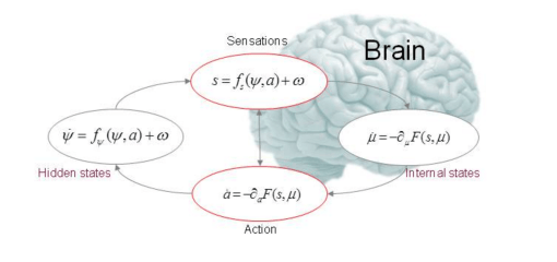
(see also the wikipedia and this 2013 review)
What are free Energies and why do we use them in Deep Learning ?
The Free Energy is a Temperature Weighted Average Energy
In (Unsupervised) Deep Learning, Energies are quadratic forms over the weights. In an RBM, one has

This is the T=0 configurational Energy, where each configuration is some 
The Free Energy 

Zero Temperature Limit
Note: as 


and only the largest term, the largest negative Energy, survives.

Other Notation
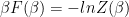
We may also see F written in terms of the partition function Z:


where the brakets 
![\mathbb{E_P}[\cdots]](https://s0.wp.com/latex.php?latex=%5Cmathbb%7BE_P%7D%5B%5Ccdots%5D+&bg=ffffff&fg=%23000000&s=0&c=20201002)

Of course, in deep learning, we may be trying to determine the distribution 
But there is more to Free Energy learning than just approximating a distribution.
The Free Energy is an average solution to a non-convex optimization problem
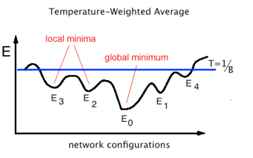
In a chemical system, the Free Energy averages over all global and local minima below the Temperature T–with barriers below T as well. It is the Energy available to do work.
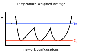
Being Scale Free: T=1
For convenience, Hinton explicitly set T=1. Of course, he was doing inference, and did not know the scale of the weights W. Since we don’t specify the Energy scale, we learn the scale implicitly when we learn W. We call this being scale-free
So in the T=1, scale free case, the Free Energy implicitly averages over all Energy minima where 
Highly degenerate non-convex problems
Because Free Energies provide an average solution, they can even provide solutions to highly degenerate non-convex optimization problems:
When do Free Energy solutions fail ?
They will fail, however, when the barriers between Energy basins are larger than the Temperature.
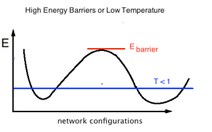
This can happen if the effective Temperature drops close to zero during inference. Since T=1 implicitly in inference, this means when the weights W are exploding.
See: Normalization in Deep Learning
Systems may also get trapped if the Energy barriers grow very large –as, say, in the glassy phase of a mean field spin glass. Or a supercooled liquid–the co-called Adam Gibbs phenomena. I will discuss this in a future post.
In either case, if the system, or solver, gets trapped in a single Energy basin, it may appear to be convex, and/or flat (the Hessian has lots of zeros). But this is probably not the optimal solution to learning when using a Free Energy method.
Free Energies produce Ruggedly Convex Landscapes
It is sometimes argued that Deep Learning is a non-convex optimization problem. And, yet, it has been known for over 20 years that networks like CNNs don’t suffer from the problems of local minima? How can this be ?
At least for unsupervised methods, it has been clear since 1987 that:
An important property of the effective [Free] Energy function E(V,0,T) is that it has a smoother landscape than E(S) [T=0] …
Hence, the probability of getting stuck in a local minima decreases
Although this is not specifically how Hinton argued for the Helmholtz Free Energy — a decade later.
The Hinton Argument for Free Energies
Why do we use Free energy methods ? Hinton used the bits-back argument:
Imagine we are encoding some training data and sending it to someone for decoding. That is, we are building an Auto-Encoder.
If have only 1 possible encoding, we can use any vanilla encoding method and the receiver knows what to do.
But what if have 2 or more equally valid codes ?
Can we save 1 bit by being a little vague ?
Stochastic Complexity
Suppose we have N possible encodings ![[h_{1},h_{2},\cdots]](https://s0.wp.com/latex.php?latex=%5Bh_%7B1%7D%2Ch_%7B2%7D%2C%5Ccdots%5D+&bg=ffffff&fg=%23000000&s=0&c=20201002)

Pick a coding with probability 

Now the receiver must guess which encoding 

where H is the Shannon Entropy of the random encoding
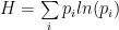
The decoding cost looks just like a Helmholtz Free Energy.
Moreover, we can use a sub-optimal encoding, and they suggest using a Factorized (i.e. mean field) Feed Forward Net to do this.
To understand this better, we need to relate
Thermodynamics and Inference
In 1957, Jaynes formulated the MaxEnt principle which considers equilibrium thermodynamics and statistical mechanics as inference processes.
In 1995, Hinton formulated the Helmholtz Machine and showed us how to define a quasi-Free Energy.
In Thermodynamics, the Helmholtz Free Energy F(T,V,N) is an Energy that depends on Temperature instead of Entropy. We need

and F is defined as

In ML, we set T=1. Really, the Temperature equals how much the Energy changes with a change in Entropy (at fixed V and N)

Variables like E and S depend on the system size N. That is,
as


We say S and T are conjugate pairs; S is extensive, T is intensive.
(see more on this in the Appendix)
Legendre Transform
The conjugate pairs are used to define Free Energies via the Legendre Transform:
Helmholtz Free Energy: F(T) = E(S) – TS
We switch the Energy from depending on S to T, where 
Why ? In a physical system, we may know the Energy function E, but we can’t directly measure or vary the Entropy S. However, we are free to change and measure the Temperature–the derivative of E w/r.t. S:
This is a powerful and general mathematical concept.
Say we have a convex function f(x,y,z), but we can’t actually vary x. But we do know the slope, w, everywhere along x

Then we can form the Legendre Transform , which gives g(w,y,z) as
the ‘Tangent Envelope‘ of f() along x

![]()

or, simply
 .
.Note: we have converted a convex function into a concave one. The Legendre transform is concave in the intensive variables and convex in the extensive variables.
Of course, the true Free Energy F is convex; this is central to Thermodynamics (see Appendix). But that is because while it is concave in T, we evaluate it at constant T.
But what if the Energy function is not convex in the Entropy ? Or, suppose we extract an pseudo-Entropy from sampling some data, and we want to define a free energy potential (i.e. as in protein folding). These postulates also fail in systems like blog post on spin chains.
Answer: Take the convex hull
Legendre Fenchel Transform
When a convex Free Energy can not be readily be defined as above, we can use the the generalized the Legendre Fenchel Transform, which provides a convex relaxation via
the Tangent Envelope , a convex relaxation
 .
.The Legendre-Fenchel Transform can provide a Free Energy, convexified along the direction internal (configurational) Entropy, allowing the Temperature to control how many local Energy minima are sampled.
Practical Applications
- This how the (TAP) Free Energy is formed for the EMF_RBM. I have written an open source version of the code in pythonopen source version of the code in python.
- Google Deep Mind released a paper in 2013 on DARN: Deep Auto Regressive Networks.
- The modeling package Edward provides Variational Inference on top of TensorFlow
- Variational AutoEncoders are available in Keras
- And it is how Jordan does Variational Inference–the topic of part II of this blog.

Happy Fourth of July
Appendix
Extra stuff I just wanted to write down…
Convexity in Thermodynamics and Statistical Physics
- S and V (or U and V) are the coordinates for the manifold of Equilibrium states
- The Energy U is a convex function of S, V, and S is concave
- The Temperature
Extensivity and Weight Constraints
If we assume T=1 at all times, and we assume our Deep Learning Energies are extensive–as they would be in an actual thermodynamic system–then the weight norm constraints act to enforce the size-extensivity.
as 
if 
and 
then W should remain bounded to prevent the Energy E(n) from growing faster than Mn. And, of course, most Deep Learning algorithms do bound W in some form.
Back to Stat Mech
 as the log sum of the number of Energy configurations, or density of states,
 (and let k = 1)
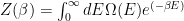
![\Omega(E)=\int_{C}d\beta e^{-\beta[E-F(\beta)]}](https://s0.wp.com/latex.php?latex=%5COmega%28E%29%3D%5Cint_%7BC%7Dd%5Cbeta+e%5E%7B-%5Cbeta%5BE-F%28%5Cbeta%29%5D%7D+&bg=ffffff&fg=%23000000&s=0&c=20201002)
where C denotes a contour integral.

Free Energy is a particular case of Massieu Characteristic Function, discovered by François Massieu and developed by Pierre Duhem. By more fundamentely, Thermodynamics and Free Energy can be linked to geometrical notion.
This history of “Characteristic Function of Massieu” could be find in the presentation:
http://forum.cs-dc.org/topic/582/fr%C3%A9d%C3%A9ric-barbaresco-symplectic-and-poly-symplectic-model-of-souriau-lie-groups-thermodynamics-souriau-fisher-metric-geometric-structure-of-information
and in the video at CIRM seminar TGSI’17:
or video of GSI’15:
http://forum.cs-dc.org/topic/291/symplectic-structure-of-information-geometry-fisher-metric-and-euler-poincar%C3%A9-equation-of-souriau-lie-group-thermodynamics-fr%C3%A9d%C3%A9ric-barbaresco
This history of Massieu is also explained in Roger Balian paper available on website of The French Academy of Science: “François Massieu et les potentiels thermodynamiques”
Click to access evol_Balian2.pdf
These structures (Legendre transform, entropy,…) are closely related to Hessian geometry developed by Jean-Louis Koszul.
Extension of Massieu Characteristic Function by Jean-Marie Souriau, called Lie Group Thermodynamics, allow to extend Free Energy on homogeneous manifolds and so also machine learning on these more abstract spaces.
Souriau Model of Lie Group Thermodynamics are developed in the first chapter of MDPI Book in papers of Marle, Barbaresco and de Saxcé:
Differential Geometrical Theory of Statistics
http://www.mdpi.com/books/pdfview/book/313
This book can be downloaded here:
http://www.mdpi.com/books/pdfdownload/book/313/1
This topic will be addressed in GSI’17 conference at Ecole des Mines de Paris in November 2017:
https://www.see.asso.fr/gsi2017
see GSI’17 program of session “Geometrical Structures of Thermodynamics”
https://www.see.asso.fr/wiki/19413_program
LikeLike
I don’t know what the dynamical group is for something like a variational auto encooder (VAE) or a deep learning model in general. In the old days, we just assumed that neural networks like MLPs proceeded by Langevin dynamics, and we did not pay much attention to the specific structure of SGD updates, the difference between dynamics and BackProp, etc. But I think there is a lot more attention being applied to the details of the update equations and what the actual dynamics are. That said, it is becoming clear, at least in VAEs, that the density has to satisfy some kind of conservation law of probability as with normalizing flows and related ideas.
LikeLike
Jean-Marie Souriau has discovered in chapter IV on “Statistical Mechanics” of his book “Structure of Dynamical Systems”, that classical Gibbs density on homogeneous (symplectic) manifold for Geometrical Mechanics is not covariant with respect to Dynamical groups of Physics (Galileo Group in classical Mechanics and Poincaré group in Relativity). Souriau has then defined a new thermodynamics, called “Lie Group Thermodynamics” where (planck) temperature is proved to be an element of the Lie algebra of the dynamical groups acting on the systems. Souriau has also geometrized the Noether theorem by inventing the “Moment map” (as an element of dual Lie algebra) that is the new fundamental preserved geometrical structure. Souriau has used this cocycle to preserve the equivariance of the action of the group on the dual Lie algebra and especially on Moment map. To convince yourself, you can read in Marle’s paper development of Souriau Lie group Thermodynamics for the most simple case “a centrifuge”:
[XX] Marle, C.-M.: From tools in symplectic and poisson geometry to J.-M. Souriau’s theories of statistical mechanics and thermodynamics. Entropy 18, 370 (2016)
http://www.mdpi.com/1099-4300/18/10/370/pdf
I have discovered that Souriau has also given a generalized definition of Fisher metric (hessian of the logarithm of Massieu’scharacteristic function) by introducing a cocycle linked with cohomology of the group. Souriau has identified Fisher metric with “geometric” calorific capacity.
Souriau gave also the good definition of Entropy, the Legendre thansform of the logarithm of Massieu’s characteristic function (related to Free Energy in new parameterization). Free Energy is not classically written in the good parameterization:
– Classical Free Energy: F=E-T.S (with S: Entropy) where F is parameterized by T.
– Free Energy should be written S=(1/T).E –F or F=(1/T).E-S where F is parameterized by (1/T).
– The good parameter is 1/T and not T, then Entropy is the Legendre transform of Free Energy in this parameterization.
– F should by parameterized by (Planck) temperature: 1/T
Souriau has generalized this relation by replacing (1/T) by the geometric temperature (element of Lie algebra) to preserve the Legendre Transform structure and the invariance of the Entropy given by this definition with respect to the action of the group. Obviously, if you consider only time translation , we recover classical thermodynamics. But it easily to prove that classical thermodynamics is not correct theory for a simple case as “thermodynamics of centrifuge” where the sub-group of Galileo group (rotation of the system along one axis) brake the symmetry and where classical Gibbs density is no longer covariant with respect to the action of this subgroup.
Souriau has geometrized Thermodynamics and has given a “Geometric Theory of Heat” (in 2018, in France, we will officially organized many events for 250th birthday of Joseph Fourier and his “heat equation”. I will present geometric heat equation of Souriau for MDPI conference in Barcelona in 2018 “From Physics to Information Sciences and Geometry”: https://sciforum.net/conference/Entropy2018-1 ; I invite you to submit a paper).
To apply this theory for Neural Network, you have to forget dynamical groups of geometric mechanics, but Souriau’s equations of “Lie Group Thermodynamics” are universal and you can apply it to make statistics of data on “homogeneous manifolds” or on “Lie groups” (you can forget the symplectic manifold, because new equations, only take into account Group and its cocycle). Especially, Neural Network on Lie Group data or time series on “Lie Group” data are more and more popular for pose recognition for instance:
[YY] Huang, Z., Wan, C., Probst, T., & Van Gool, L. (2016). Deep Learning on Lie Groups for Skeleton-based Action Recognition. arXiv preprint arXiv:1612.05877.
[ZZ] Learning on distributions, functions, graphs and groups, Workshop at NIPS 2017, 8th December 2017; https://sites.google.com/site/nips2017learningon/
With Souriau definition of Fisher Metric, you can extend classical “Natural Gradient” (from Information Geometry) on abstract spaces , for learning from data on homogeneous manifold and Lie Group. Then, the invariance by reparametrization of “Natural gradient” is replaced by invariance by all symmetries (Gibbs density is made covariant with respect to the group acting transitively on the homogeneous manifolds and Fisher metric of backpropagation “Natural Gradient” is invariant with respect to the group). To have more details on Geometric approach of Natural Gradient (Riemannian Neural Networks), see Yann Ollivier papers (http://www.yann-ollivier.org/rech/index_chr ) written at Paris-Saclay University or his lecture at “Collège de France”:
[AA] Yann Ollivier, Riemannian metrics for neural networks I: Feedforward networks, Information and Inference 4 (2015), n°2, 108–153; http://www.yann-ollivier.org/rech/publs/gradnn.pdf
[BB] Yann Ollivier, Gaétan Marceau-Caron, Practical Riemannian neural networks, Preprint, arxiv.org/abs/1602.08007 ; http://www.yann-ollivier.org/rech/publs/riemaNN.pdf
About Langevin Dynamics, based on Paul Langevin equation, we can mix natural gradient and Langevin Dynamics to define a “Natural Langevin Dynamics” as published by Yann Ollivier in GSI’17:
[CC] Yann Ollivier and Gaétan Marceau Caron. Natural Langevin Dynamics for Neural Networks, GSI’17 Geometric Science of Information, Ecole des Mines ParisTech, Paris, 7th-9th November 2017.
https://www.see.asso.fr/wiki/19413_program
Mixing Langevin Dynamics with Souriau-Fisher Metric will provide a new backpropagation based on “Symplectic Integrator” that have all good properties of invariances in the framework of calculus of variations and Hamiltonian formalisms.
I have recently observed that with Souriau Formalism, Gaussian density is a maximum entropy of 1rst order (see tensorial notation and parameterization of multivariate Gaussian by Souriau) and not a 2nd order. We can then extend Souriau model with polysymplectic geometry to define a 2nd order maximum entropy Gibbs density in Lie Group Geometry , useful for “small data analytics”. I will present this paper at GSI’17:
[DD] F. Barbaresco, Poly-Symplectic Model of Higher Order Souriau Lie Groups Thermodynamics for Small Data Analytics, GSI’17 Geometric Science of Information, Ecole des Mines ParisTech, Paris, 7th-9th November 2017.
https://www.see.asso.fr/wiki/19413_program
To conclude, Free Energy is a fundamental structure, but just a particular case of Massieu’s characteristic function. We need to geometrize Thermodynamics in Geometric Mechanics but also for Machine Leaning with neural networks on data belonging to homogeneous manifolds or Lie Groups. For the generalization, Souriau’s Lie Group Theory is the right model. We can prove that there is no other ones. In Information geometry, and in the case of exponential families, the fundament group is the “general affine group”. The geometry is in the case related to co-adjoint orbits of this group. Using Souriau-Konstant-Kirilov 2 form, we can then rediscover a symplectic geometry associated to these co-adjoint orbits.
These concepts are now very classical in Europe, and are developed in GSI (Geometric Science of Information) or TGSI (Topological & Geometrical Structures of Information) conferences. We can no longer ignore them.
With European actors of Geometric Mechanics, we have just submitted a project to the European commission to use these new geometric structures to make recommendation for designing new generation of HPC (High Power Computer) Machine that could beneficiate of symmetries preservation. We will replace “Pascaline” machine (invented by Blaise Pascal under the influence of Descartes) and its more recent avatars (until GOOGLE TPU) that are coordinate-dependent to new generation “Lie Group” machines based on Blaise Pascal “Aleae Geometria” (geometrization of probability) that will be coordinate-free-dependent and intrinsic without privilege coordinate systems.
Frederic Barbaresco
GSI’17 Co-chairman
http://www.gsi2017.org
LikeLike