Normalization in Deep Learning

A few days ago (Jun 2017), a 100 page on Self-Normalizing Networks appeared. An amazing piece of theoretical work, it claims to have solved the problem of building very large Feed Forward Networks (FNNs).

It builds upon a Batch Normalization (BN), introduced in 2015– and is now the defacto standard for all CNNs and RNNs. But not so useful for FNNs.

What makes normalization so special? It makes very Deep Networks easier to train, by damping out oscillations in the distribution of activations.

To see this, the diagram below uses data from Figure 1 (from the BN paper) to depict how the distribution evolves for a typical node outputs in the last hidden layer of a typical network:

node outputs, with and without Batch Normalization

Very Deep nets can be trained faster and generalize better when the distribution of activations is kept normalized during BackProp.

We regularly see Ultra-Deep ConvNets like Inception, Highway Networks, and ResNet. And giant RNNs for speech recognition, machine translation, etc. But we don’t see powerful Feedforward Neural Nets (FNNS) with more than 4 layers. Until now.

Batch Normalization is great for CNNs and RNNs.

But we still can not build deep MLPs

This new method — Self-Normalization — has been proposed for building very deep MultiLayer Perceptions (MLPs) and other Feed Forward Nets (FNNs).

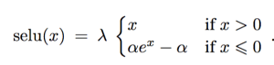
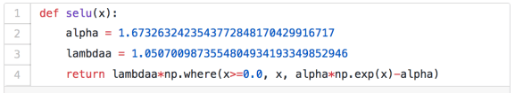
The idea is just to tweak a the Exponential Linear Unit (ELU) activation function to obtain a Scaled ELU (SELU):

With this new SELU activation function, and a new, alpha Dropout method, it appears we can, now, build very deep MLPs. And this opens the door for Deep Learning applications on very general data sets. That would be great!

The paper is, however, ~100 pages long of pure math! Fun stuff.. but a summary is in order.

I review Normalization in Neural Networks, including Batch Normalization, Self-Normalization, and, of course, some statistical mechanics (it’s kinda my thing).

This is an early draft of the post: comments and questions are welcome

Setup

WLOG, consider an MLP, where we call the input to each layer u

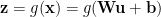
The linear transformations at each layer is

$\mathbf{x}=\mathbf{Wu}+\mathbf{b}$ ,

and we apply standard point-wise activations, like a sigmoid

$g(\mathbf{x}_{i})=\dfrac{1}{1+exp(-\mathbf{x}_{i})}$

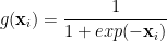
so that the total set of activations (at each layer) takes the form

$\mathbf{z}=g(\mathbf{x})=g(\mathbf{Wu}+\mathbf{b})$

The problem is that during SGD training, the distribution of weights W and/or the outputs x can vary widely from iteration to iteration. These large variations lead to instabilities in training that require small learning rates. In particular, if the layer weights W or inputs u blow up, the activations can become saturated:

$as\;\;\Vert\mathbf{W}\Vert\rightarrow\infty,\;\;\;g(\mathbf{x})\rightarrow 0$ ,

leading to vanishing gradients. Traditionally, this was in MLPs avoided by using larger learning rates, and/or early stopping.

One solution is better activation functions, such as a Rectified Linear Unit (ReLu)

$g(\mathbf{x}_{i})=max(\mathbf{x}_{i},0)$

or, for larger networks (depth > 5), an Exponential Linear Unit (ELU):

Which look like:

Indeed, sigmoid and tanh activations came from early work in computational neuroscience. Jack Cowan proposed first the sigmoid function as a model for neuronal activity, and sigmoid and tanh functions arise naturally in statistical mechanics. And sigmoids are still widely used for RBMs and MLPs–ReLUs don’t help much here.

Note: ReLUs only help Deep CNNs and RNNs

SGD training introduces perturbations in training that propagate through the net, causing large variations in weights and activations. For FNNs, this is a huge problem. But for CNNs and RNNs..not so much. why ?

CNNs and RNNs, are less distorted by the SGD perturbations–presumably because of their weight sharing architectures.
LSTMs also avoid this problem by replacing multiplies with additions.
Moreover, Dropout (a stochastic regularizer) works very well with ReLUs in CNNs and RNNs, but not so much for MLPs and other FNNs.
And very Deep Nets, like ResNet, which have > 150 layers, use skip connections to help propagate the internal residuals.

It has been said the no real theoretical progress has been made in deep nets in 30 years. That is absurd. We did not have ReLus or ELUs. In fact, up until Batch Normalization, we were still using SVM-style regularization techniques for Deep Nets. It is clear now that we need to rethink generalization in deep learning.

Max-Norm Constraints

We can regularize a network, like a Restricted Boltzmann Machine (RBM), by applying max norm constraints to the weights W.

This can be implemented in training by tweaking the weight update at the end of pass over all the training data

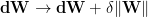
$\mathbf{dW}\rightarrow\mathbf{dW}+\delta\Vert\mathbf{W}\Vert$

where $\Vert\mathbf{W}\Vert$ is an L1 or L2 norm.

I have conjectured that this is actually kind of Temperature control, and prevents the effective Temperature of the network from collapsing to zero.

$as\;\;\Vert\mathbf{W}\Vert\rightarrow\infty,\;\;\;T^{eff}\rightarrow 0\;$ ,

By avoiding a low Temp, and possibly any glassy regimes, we can use a larger effective annealing rate–in modern parlance, larger SGD step sizes.

It makes the network more resilient to changes in scale.

After 30 years of research neural nets, we can now achieve an analogous network normalization automagically.

But first, what is current state-of-the-art in code ? What can we do today with Keras ?

Batch Normalization (BN) Transformation

Tensorflow and other Deep Learning frameworks now include Batch Normalization out-of-the-box. Under-the-hood, this is the basic idea:

At the end of every mini-batch $\mathcal{B}_{k}$ , the layers are whitened. For each node output x (and before activation):

$\hat{\mathbf{x}}_{k}=\mathbf{Wu}_{k}+\mathbf{b}_{k}$

the BN Transform maintains the (internal) zero mean $\mu_{\mathcal{B}}=0$ and unit variance ( $\sigma^{2}_{\mathcal{B}}=1$ ).

We evaluate the sample mini-batch mean and variance , and then normalize, scale, and shift the values:

The final transformation is applied inside the activation function g():

$g(BN(\mathbf{x}))=g(\mathbf{y}))$

although we can absorb the original layer bias term b into the BN transform, giving

$g(BN(\mathbf{x}))=g(BN(\mathbf{Wu}))$

So now, instead of renormalizing the weights W after passing over all the data, we can normalize the node output x=Wu explicitly, for each mini-batch, in the BackProp pass.

Note that

$\Vert\mathbf{Wu}\Vert<\Vert\mathbf{W}\Vert\Vert\mathbf{u}\Vert$

so bounding the weights with max-norm constraints got us part of the way already.

Note that extra scaling and shift parameters $(\gamma,\beta)_{k}$ appear for each batch (k), and it is necessary to optimize these parameters as a side step during training.

At the end of the transform, we can normalize the network outputs (shown above) of the entire training set (population)

$\mathbf{\hat{x}}=\dfrac{\mathbf{x}-\mathbb{E}[\mathbf{x}]}{\sqrt{Var[\mathbf{x}]+e}}$ ,

where the final statistics are computed as, say, an unbiased estimate over all (m) mini-batches of the training data

$Var[\mathbf{\hat{x}}]=\dfrac{m}{m-1}\mathbb{E}_{\mathbb{B}_{m}}[\sigma^{2}_{\mathbb{B}_{m}}]$ .

Benefits of the Batch Norm Transform

The key to Batch Normalization (BN) is that:

the statistics are gathered during a mini-batch step
the normalization can be integrated directly into backprop
the extra parameters can be tuned during training

BN allows us to manipulate the activation function of the network. It is a differentiable transformation that normalizes activations in the network.

It makes the network (even) more resilient to the parameter scale.

It has been known for some time that Deep Nets perform better if the inputs are whitened. And max-norm constraints do re-normalize the layer weights after every mini-batch.

Batch normalization appears to be more stable internally, with the advantages that it:

has replaced max norm constraints
is implemented directly in BackProp
has larger learning rates with standard solvers => faster convergence
replaces / augments Dropout as a regularizer

Still, Batch Norm training slows down BackProp. Can we speed it up ?

Self-Normalizing Activations

A few days ago, the Interwebs was buzzing about the paper Self-Normalizing Neural Networks. HackerNews. Reddit. And my LinkedIn Feed.

These nets use Scaled Exponential Linear Units (SELU), which have implicit self-normalizing properties. Amazingly, the SELU is just a ELU multiplied by $\lambda$

Screen Shot 2017-06-14 at 5.05.10 PM

where $\lambda>1$ .

The paper authors have optimized the values as:

Screen Shot 2017-06-16 at 7.39.49 PM

**a comment on reddit suggests tanh may work as well

The SELUs have the explicit properties of:

negative and positive values for controlling the mean $\mu$
saturation regions to dampen the variance $\sigma$ if it is too large in the lower layer,
a slope > 1 to increase $\sigma$ if it is too small in the lower layer, and
a continuous curve, which ensures a fixed point.

Amazingly, the implicit self-normalizing properties are actually proved–in only about 100 pages–using the Banach Fixed Point Theorem.

They show that, for an FNN using selu(x) actions, there exists a unique attracting and stable fixed point for the mean and variance. (Curiously, this resembles the argument that Deep Learning (RBMs at least) the Variational Renormalization Group (VRG) Transform.

There are, of course, conditions on the weights–things can’t get too crazy. This is hopefully satisfied by selecting initial weights with zero mean and unit variance.

$\sigma^{2}_{\mathcal{B}}=1\;or\; \dfrac{1}{\sqrt{N}}$ ,

(depending how we define terms).

To apply SELUs, we need a special initialization procedure, and a modified version of Dropout, alpha-Dropout,

SELU Initialization

We select initial weights $\mathbf{W}$ from a Gaussian distribution with mean 0 and variance $\frac{1}{\sqrt{N}}$ , where N is number of weights:

Screen Shot 2017-06-16 at 8.08.30 PM — TensorFlow implementation of Weight Initialization

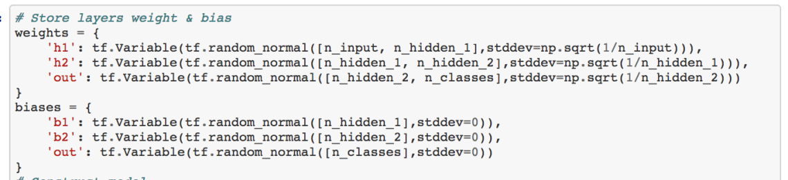
In Statistical Mechanics, this the Temperature is proportional to the variance of the Energy, and therefore sets the Energy scale. Since E ~ W,

SELU Weight initialization is similar in spirit to fixing T=1.

Alpha Dropout

Note that to apply Dropout with an SELU, we desire that the mean and variance are invariant.

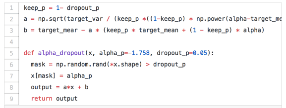
We must set random inputs to saturated negative value of SELU, $\alpha\lambda$ Then, apply an affine transformation, computing relative to dropout rate.

Screen Shot 2017-06-16 at 7.40.40 PM

(thanks to ergol.com for the images and discussion).

All of this is provided, in code, with implementations already on github for Tensorflow, PyTorch, Caffe, etc. Soon…Keras?

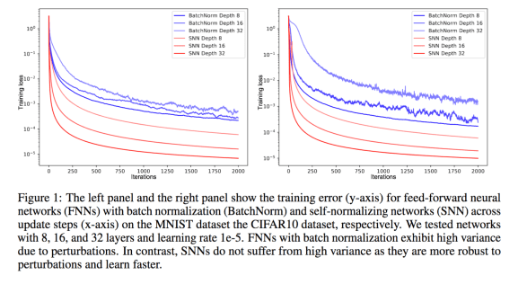
Key Results

The key results are presented in Figure 1 of the paper, where SNN = Self Normalizing Networks, and the data sets studies are MNIST and CIFAR.

The original code is available on github

Great discussions on HackerNews and Reddit

Summary

We have reviewed several variants of normalization in deep nets, including

Max Norm weight constraints
Batch Normalization, and
Self-Normalizing, Deep Feed Forward Nets

Along the way, I have tried to convince you that recent developments in the normalization of Deep Nets represent a culmination over 30 years of research into Neural Network theory, and that early ideas about finite Temperature methods from Statistical Mechanics have evolved into and are deeply related to the Normalization methods employed today to create very Deep Neural Networks

Appendix:

Temperature Control in Neural Networks

Very early research in Neural Networks lifted idea from statistical mechanics. Early work by Hinton formulated AutoEncoders and the principle of the Minimum Description Length (MDL) as minimizing a Helmholtz Free Energy:

$F=U-TS$ ,

where the expected (T=0) Energy is

$U=\sum\limits_{i}p_{i}E_{i}$ ,

S is the Entropy,

and the Temperature $T=\dfrac{1}{\beta}=1$ implicitly.

Minimizing F yields the familiar Boltzmann probability distribution

$latex p_{i}=\dfrac{e^{-\beta E_{i}}}{\sum\limits_{j}e^{-\beta E_{j}}}&bg=ffffff $.

When we define an RBM, we parameterize the Energy levels $E_{i}$ in terms of the configuration of visible and hidden units $(i\rightarrow\mathbf{u},\mathbf{v})$

$E(\mathbf{v},\mathbf{h})=\mathbf{b^{T}v}+\mathbf{c^{T}h}+\mathbf{h^{T}Wv}$ ,

giving the probability

$P(\mathbf{v},\mathbf{h})=\dfrac{e^{-\beta E}}{Z(\beta)}$

where $Z(\beta)$ is the Partition Function, and, again, T=1 implicitly.

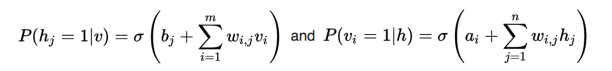
In Stat Mech, we call RBMs a Mean Field model because we can decompose the total Energy and/or conditional probabilities using sigmoid activations $\sigma()$ for each node

Screen Shot 2017-06-14 at 11.31.33 PM

In my 2016 MMDS talk, I proposed that without some explicit Temperature control, RBMs could collapse into a glassy state.

And now, some proof I am not completely crazy:

Another recent 2017 study on the Emergence of Compositional Representations in Restricted Boltzmann Machines, we do indeed see that the RBM effective Temperature does indeed drop well below 1 during training

$T^{eff}<<1$

and that RBMs can exhibit glassy behavior.

I also proposed that RBMs could undergo Entropy collapse at very low Temperatures. This has also now been verified in a recent 2016 paper.

Finally, this 2017 paper:Train longer, generalize better: closing the generalization gap in large batch training of neural networks” proposes that many networks exhibit something like glassy behavior described as “ultra-slow” diffusion behavior.

Sketch of the Proof:

I will sketch out the proof in some detail if there is demand. Intuitively (& citing comments in HackerNews): ”

“for negative net inputs the variance is decreased, for positive net inputs the variance is increased.
for very negative values the variance decrease is stronger. For inputs close to zero the variance increase is stronger.
for large invariance in one layer, the variance gets decreased more in the next layer, and vice versa.
Theorem 2 states that the variance can be bounded from above and hence there are not exploding gradients.
Theorem 3 states that the variance can be bounded from below and does not vanish.”