Is your layer over-fit? (part 2)

Say you are training a Deep Neural Network (DNN), and you see your model is over-trained. Or just not performing well. Is there a way to detect which layer is actually over-trained? (or over-fit, as some people call it)

In this post, we will show how to use the open-source weightwatcher tool to answer this.

WeightWatcher is an open-source, data-free diagnostic tool for analyzing (pre-)trained DNNs. It is based on my personal research into Why Deep Learning Works, in collaboration with UC Berkeley. It is based on ideas from the Statistical Mechanics of Learning (i.e theoretical physics and chemistry).

pip install weightwatcher

WeightWatcher lets you inspect your layer weight matrices to see if they are converging properly. And in some cases, it can even tell you if the layer is over-trained. The idea is simple. If you are training a model, and you over-regularize one of the layer, then you any observe the weightwatcher alpha metric drops below 2 (). This is predicted by our HTSR theory of learning (although we have not published this specific result yet). And very unique as no other approach can do this.

To see how this works, we will look at a very specific, carefully-designed experiment where the theory is known to work exactly as advertised.

BUT (and here’s the disclaimer)

Please be aware–training DNNs to State-of-the-Art (SOTA) is not easy, and applying the tool requires designing careful experiments that can isolate the problems you are trying to fix. It does not work in every case, and you may see unusual results that are difficult to interpret. In these cases, please feel free to reach out to me directly to get help.

Having said that, let’s get started

HERES THE GOOGLE COLAB NOTEBOOK

Experimental Design

We consider a very simple DNN, a 3-layer MLP (Multi-Layer Perceptron), trained on MNIST.

To induce the overtraining, we will train this model using different batch sizes, with batch_size in [1,2,4,8,16,32].

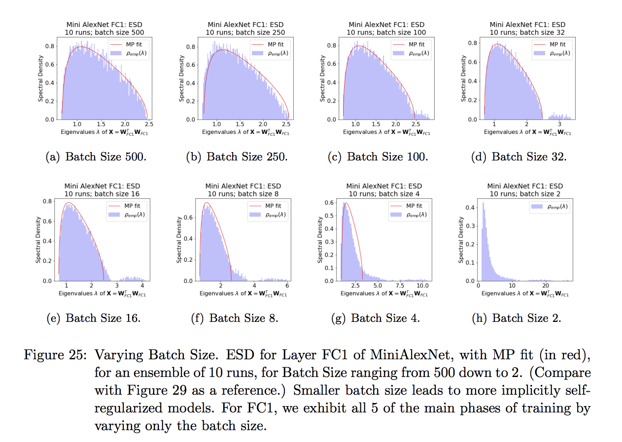
Why do we vary the batch sizes ?… and not a specific regularization hyper-parameter like Weight Decay or Dropout? The batch size acts like a very strong regularizer, which can induce the Heavy-Tails we see in SOTA models even in this very small model and generally poorly performing model. This is shown in Figure 25 of our JMLR paper describing our theory of Heavy-Tailed Self-Regularization (HT-SR), the theory behind weightwatcher.

Moreover, with extremely small batch sizes, and a long number of epochs, we can even drive the model into a state of over-training. Which is the goal here.So each model is trained for a very long number of epochs, and until the training loss stabilizes, using a Keras EarlyStopping Callback

tf.keras.callbacks.EarlyStopping(monitor='loss', patience=3, verbose=0, min_delta=0.001, restore_best_weights=True)e()

In your own models, the situation may be more complex.

The weightwatcher metrics work best when applied to SOTA models because this is when the layer weight matrics are best correlated, and the Power Law fits work the best. It takes some work to design experiments on small models that can flush out these features. So we choose to use the batch size to induce this effect. But let me encourage you to try other approaches.

The key to using the HTSR theory is to carefully control the training so that when you adjust some other knob (i.e Dropout, momentum, weight decay) that the training and test error change smoothly and systematically. If, however, the training accuracy or loss is unstable, and you are jumping all over the loss landscape, then HTSR theory, is more difficult to apply. So, here,

I follow the KISS mantra: “Keep It Super Simple!”

Reproducibility

To compare 2 or more models to each other, with different batch sizes, for the purposes here, we need to ensure they have been trained with the exact same initial conditions. To do this, we have to both set all the random seeds to a default value and tell the framework (here, Keras) to use deterministic options. This also, nicely, makes the experiments 100% reproducible.

%env CUBLAS_WORKSPACE_CONFIG=:4096:8

import random
def reset_random_seeds(seed_value=42):
   os.environ['PYTHONHASHSEED']=str(seed_value)
   tf.random.set_seed(seed_value)
   tf.keras.utils.set_random_seed(seed_value)
   np.random.seed(seed_value)
   random.seed(seed_value)
   tf.config.experimental.enable_op_determinism()

Every time we build the model, we will first run reset_random_seeds()to ensure that every run, with different batch sizes, regularization, etc, is stated from the same spot and is reproducible.

Model Size and Shape: The Three (3) Layers

This model has 3 layers: input, hidden, and output. Note that each layer is initialized in the same way (i.e with GlorotNormalization, with the same seed). Also, here, to keep it super simple, no specific regularization is applied to the model (except for the changing of the batch size).

initializer = tf.keras.initializers.GlorotNormal(seed=1)
  model = tf.keras.models.Sequential([
      tf.keras.layers.Flatten(input_shape = [28,28]),
      tf.keras.layers.Dense(300, activation='relu', kernel_initializer=initializer),
      tf.keras.layers.Dense(100, activation='relu', kernel_initializer=initializer),
      tf.keras.layers.Dense(10, activation='softmax', kernel_initializer=initializer),
  ])escribe()Also, 

We can inspect the model using weightwatcher to see how the layers are labeled (layer_id), what kind of layer they are (DENSE, Conv2D, etc), and what their shapes are (N, M).

import weightwatcher as ww
watcher = ww.WeightWatcher(model=model)
watcher.describe()

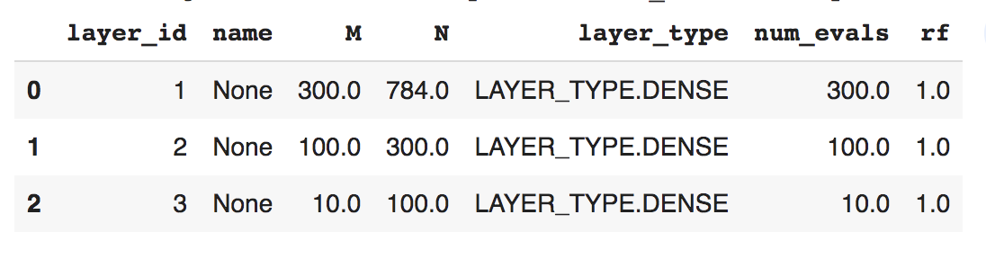
In this experiment, we will analyze layer 1 (the Hidden Layer) and only layer 1. This layer is a DENSE layer, which has a single weight matrix of dimension 100×300. It will have 100 eigenvalues, which is a large enough size for weightwatcher to analyze. And for this super, simple experiment, this is the only later that is trainable; all other layers are held fixed.

Training the model (with different batch sizes)

Again, we will train the same model, with the same exact same initial conditions, in a deterministic way, while changing the batch size. For each fully trained model, we then compute the weighwatcher Power-Law capacity metric alpha (). We will then compare the layer 1 alpha ) to the model test accuracy for each run.

Notice first that, however, when decreasing the batch size, both the training accuracy and the test accuracy improve both smoothly and systematically, and then drop off suddenly. For example, below, see that test accuracy increases from 89.0% at batch size 32 to 89.4% at batch size 4, and then drops off suddenly for batch size 2 down to 88.5%. (The training accuracy behaves in a similar way when decreases the batch size, as can be seen in the notebook).

Likewise, the training loss is varying smoothly, and the optimizer is not jumping all over the energy landscape. This indicates a clean experiment, amenable to analysis.

(Notice that we apply early stopping to the training loss, not the validation loss. That is because, in this experiment, we are trying to drive the model to a state of over-training by reducing the batch size, and going past the perhaps more common early stopping critera on the validation loss. Also, since we are changing the batch size, we want to ensure each model runs with enough epochs to the runs can be compared to each other).

The WeightWatcher Layer Capacity Matric Alpha ()

To compute the weightwatcher metrics, at the end of every training cycle, just run

results = watcher.analyze(layers=[1])

The watcher.analyze() method will generate a pandas dataframe, with layer by layer metrics.

What does alpha mean? Alpha () is a measure of how Heavy-Tailed the layer is. It can be found, crudely, by simply plotting a histogram of the eigenvalue of the layer correlation matrix, X=np.dot(W.T,W), on a log-log scale, and calculating the slope of this plot in the tail region. Here is an example where .

The smaller alpha is, the more Heavy-Tailed the layer matrix X is, and the better the layer performs for the model. But only upto a point. If the layer is too Heavy-Tailed, where (for simple models) then it may be over-trained.

Results: detecting an over-trained layer

We can now plot the alpha vs the test accuracy for layer 1, and the result is quite amazing.

Notice 2 key things

• as the test accuracy increases, the alpha metric decreases ()
• as soon the test accuracy drops (with batch size = 1), alpha drops below 2 ()

For simple models like this 3-layer MLP, the weightwatcher approach can, remarkably, detect which layer is over-trained! No other theory can do this.

For more complex models, with lots of parameters varying, the situation may be more complex.

Let me encourage you to try the weightwatcher tool for yourself, and join our Slack channel to discuss this and other aspects of training large models to SOTA.

Why does alpha < 2 mean the layer may be over-trained ?

The weightwatcher alpha $(latex \alpha)$ metric is the exponent found when fitting the empirical spectral density (ESD), or a histogram of the eigenvalues, to a Power-Law distribution. Moreover, when alpha is between roughly 2 and higher (theoretically 4, practically, upto 6, ), as shown in our JMLR paper, we can use our HTSR theory to characterize the layer weight matrix as being Moderately Heavy-Tailed. See Table 1:

When a Power Law distribution is simply Moderately Heavy-Tailed, this means that, in the limit, the variance may be unbounded, but the average (or mean) value is well defined. So, for Deep Learning, this implies that the model has learned a wide variety of correlations, but, on average, the correlations are reasonably bounded, moreover, typical. Being typical, the layer weight matrix model can be used to describe the information in the training and the test data, as long as they come from the same data distribution,

But when the alpha is very small (), this means the layer weight matrix is Very Heavy-Tailed, and the layer weight matrix is atypical. That is, the distributions of the correlations do not have a well-defined average of mean value, and the individual elements of W may even themselves be unbounded (ie. when you have a Correlation Trap). Therefore, this layer weight matrix can not be used to describe any data except the training data.

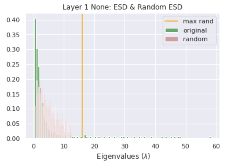
A Correlation Trap appears when the batch size = 1

Seeing this in practice is not necessarily easy, and interpreting it is harder. As here, one may have to design a very careful experiment to flush this out. Still, we encourage you to try the tool out, try to use it to identify and resolve such problems, and please give feedback.

Final Plug

And if you need help with AI, ML, or just Data Science, please reach out. I provide strategy consulting, data science leadership, and hands-on, heads-down development. I will have availability in Q3 2022 for new projects. Reach out today. #talkToChuck #theAIguy