What is WeightWatcher ?
The WeightWatcher tool is an open-source python package that can be used to predict the test accuracy of a series similar of Deep Neural Network (DNN) — without peeking at the test data.
WeightWatcher is based on research done in collaboration with UC Berkeley on the foundations of Deep Learning. We built this tool to help you analyze and debug your Deep Neural Networks.
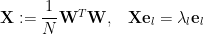
It is easy to install and run; the tool will analyze your model and return both summary statistics and detailed metrics for each layer:
The WeightWatcher github page lists various papers and online presentations given at UC Berkeley and Stanford, and various conferences like ICML, KDD, etc. There, and on this blog, you can find examples of how to use it.
This post describes how to select the metric for your models, and why.
Different Metrics for Different Models
You can use WeightWatcher to model a series of DNNs of either increasing size, or with different hyperparameters. But you need different metrics — 

- alpha
: for different hyper-parameters settings (batch size, weight decay, …) on the same model
- weighted alpha:
: for an architecture series like VGG11, VGG13, VGG16, VGG19
But why do need 2 different alpha metrics? To understand this, we need to understand
Spectral Norms and Deep Learning
Traditional machine learning theory suggests that the test performance of a Deep Neural Network is correlated with the average log Spectral Norm. That is, the test error should be bounded by the average Spectral Norm, so the smaller norm, the smaller the test error.
The Spectral Norm 


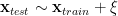
We denote the (squared) Spectal Norm as:

Note: in earlier papers we (and others) also use: 
WeightWatcher computes the log Spectral Norm for each layer, and defines:

which we compute by averaging over all 
We compute the eigenvalues, or the Empirical Spectral Density (ESD), of each layer 
Spectral Norm Regularization
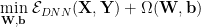
It has been suggested by Yoshida and Miyato that the Spectral Norm would make a good regularizer for DNNs. The basic idea is that the test data should look enough like the training data so that if we can say something about how the DNN performs on perturbed training data, that will also say something about the test performance.
Here is the text from the paper; let. me explain how to interpret this in practical terms.

We imagine the test data 


As we train a DNN, we run several epochs of BackProp, which amounts to multiplying


To get an estimate, or bound, on the test accuracy, we can then imagine applying the matrix multiply to the perturbed training point

So if we can say something about how the DNN should perform on a perturbed training point 

What can we say ?
When we apply an activation function 

So we say that we want to learn a DNN model such that, at each layer, the action of the layer matrix-vector multiply is bounded by the Spectral Norm of its layer weight matrix. This should, in theory, give good test performance. By applying a Spectral Norm regularizer, we think we can make a DNN that is more robust to small changes in it’s input. That is, we can make it perform better on random perturbations the of training data , and, therefore, presumably, better on the test data.
From Bounds to a Regularizer
When we develop a mathematical bound , our first instinct is to develop a numerical regularizer 

Notice that since the regularizer
A regularizer must also be easy to implement. For example, we could also bound the Jacobian 


Also, since this expression is linear in
Spectral Norm Regularization has not been widely used (outside say GANs) because it only works well for very deep networks. See, however, this adaption for smaller DNNs called Mean Spectral Normalization.
From Worst-Case Bounds to Average Case Behavior
What do we want from a theory of learning ? With WeightWatcher, we have never sought. a rigorous bound. That’s not the goal of our theory. We do not seek a bound because this decribes the worst-case behavior; we seek to understand the average-case behavior (However, what we can do repair the Spectral Norm as a metric , as shown below.)
With the average-case, we hope to able to predict the generalization error of a DNN (and without peeking at the test data). And we mean this a very practical sense, applying to very large, production quality models, both in training and fine-tuning them.
So what’s the difference between having a bound and analyzing average-case behavior ?
- With a mathematical bound, we can bound the error–for a single model. So this is alike a prediction, and , as shown above, we can use this to develop better regularizers.
- WIth the average-case behavior, we want to predict trends across many different models. Of both different depths (since deeper models usually perform better) and with different hyperparameter settings (batch size, momentum, weight decay, etc.)
It’s not at all obvious that we can expect a mathematical bound to be correlated with trends in the test accuracy of real-world DNNs. It turns out, the Spectral Norm works pretty well–at least across pretrained DNNs of increasing depth.
Here is an example, showing how the Spectral Norm performs on the VGG series

(VGG11, VGG13, VGG16, VGG19, with/out Batchnorm, trained on Imagenet-1K)
We see that the average log Spectral norm correlates quite well with the test accuracy of the DNN architecture series of the pretrained VGG models. This is remarkable, since we do not have access to the training or the test data (or other information).
We have used WeightWatcher to analyze hundreds of pretrained models, of increasing depths, and using different data sets. Generally speaking, the average log Spectral Norm correlates well with the test accuracies of many different DNN series and for different data sets.
But not always. And that’s the rub.
Simpson’s Paradox (or our Spectral surprise)
Oddly, while the average log Spectral Norm 
We have noted this, and it has also pointed by Bengio and co-workers. Indeed, an entire contest was recently set up to study this issue–the 2020 NeurIPS Predicting Generalization challenge.
Below we can see the paradox by looking at predictions for ~100 small, pre-trained VGG-like models, (provided by contest). We use WeightWatcher (version ww0.4) to compute the average log_spectral_norm, and compare to. the reported test accuracies for the contest task2_v1 set of baseline VVG-like models:
For more details, please see the contest website details, and/or our contest post-mortem Jupyter Book and paper on the contest (coming soon).
Notice that the 2xx models have the best test accuracies, and, correspondingly, as a group, the smallest avg logspectralnorm. Smaller error correlates with the smaller norm metric. Likewise, the 6xx models models have. the smallest Test Accuracies as. a group, and also, the largest avg logspectralnorm.

This is a classic example of Simpson’s Paradox.
However, also note that, for each model group (2xx, 10xx, 6xx, & 9xx), we can draw, roughly, a straight line that shows most of the test accuracies in that group are anti-correlated with the avg. log_spectral_norm
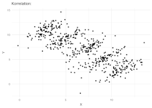
This is a classic example of Simpon’s Paradox.
Here, we see a large trend, across the similar models, trained on the same dataset, but with different, depths.
When looking closely at each model group, however, we see the reverse trend.
This makes the Spectral Norm difficult to use as a general purpose metric for predicting test accuracies.
WeightWatcher to the Rescue
Using WeightWatcher, however, we can repair the average log Spectral Norm metric by computing it as a weighted average–weighted by the WeightWatcher
Here is a similar plot on the same task2_v1 data,, but this time reporting the WeightWatcher average power law metric

WeightWatcher alpha tells us how correlated a single DNN model is. And we can use to correct the average log_spectral_norm by simply taking a weighted average (called alpha_weighted):

If we look closely, we can see more in more detail how the weighted alpha log_spectral_norm metric in the VGG architecture series. Below we use WeightWatcher to plot the different metrics vs. the Top 1 Test Accuracy for the many different pre-trained VGG models.
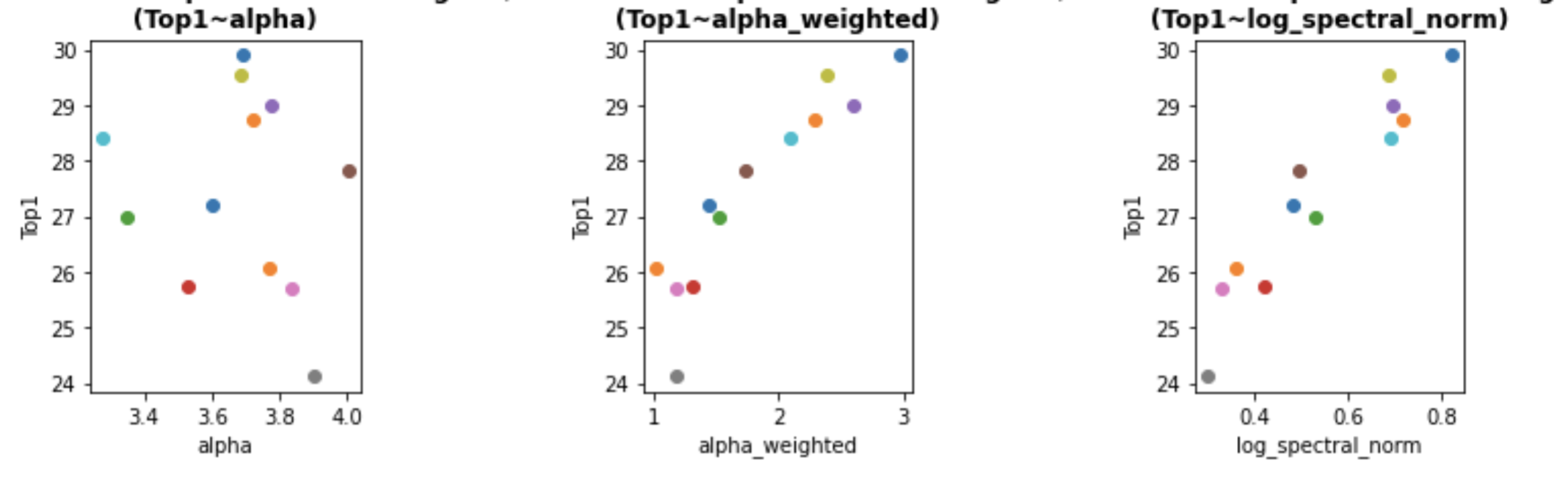
(VGG11, VGG13, VGG16, VGG19, with/out BatchNorm, trained on Imagenet-1K)
Consider the plot on the far right, and, specifically, the pink (BN-VGG-16) and red dots (VGG-19), near test accuracy ~ 26. These are 2 models with both different depths (16 vs 19 layers) and different hyperparameter settings (BatchNorm or not). The two models have nearly the same accuracy, but a large variance between their average log_spectral_norm. Now consider the far left plot for average alpha 
alpha_weighted metric corrects the average log_spectral_norm, reducing the variance between similar models, and making
Summary
The open source WeightWatcher tool provides metrics for Deep Neural Networks that allow the user to predict (trends in) the test accuracies of Deep Neural Networks without needing the test data. The different (power law) metrics,
The
The
To explain why 
While theory suggests that
We show that we can fix-up the average log_spectral_norm (as provided in WeightWatcher) by using a weighted average, weighted by the WeightWatcher power-law layer alpha alpha_weighted:
Try it yourself on your own DNN models.
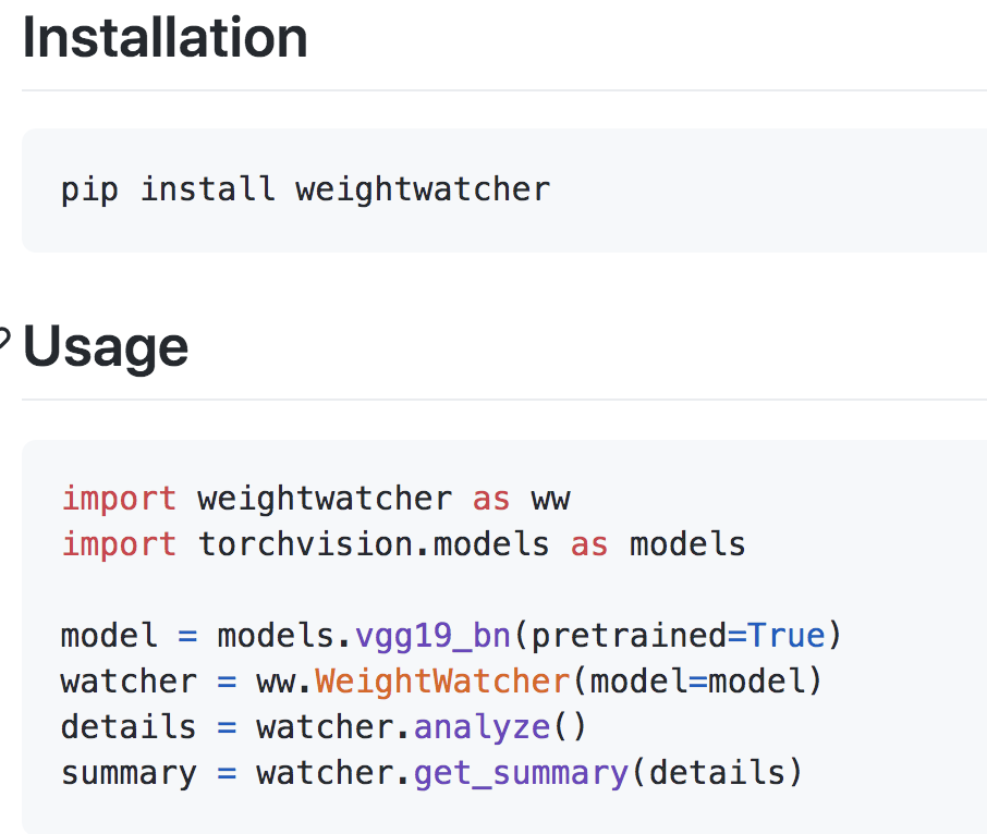
pip install weightwatcher
And let me know how it goes.
Appendix
Spectral Density of 2D Convolutional Layers
We can test this theory numerically using WeightWatcher. Notice, however, that while it is obvious how to define
WeightWatcher has 2 methods for computing the SVD of a Conv2D layer, depending on the version. For a 
- new version ww.0.4: extract
matrix slices of dimension
matrix, and run SVD on this. This gives 1 ESD per Conv2D layer.
- old version ww2x: extract
of dimension
- future version (maybe): Run SVD on the linear operator that defines the Conv2D transform. This requires running SVD on the discrete FFT on each of the Conv2D input-output channels, and then combining the resulting eigenvalues into 1 very large ESD. This is quite slow and the numerical results were not as good in early experiments.
All three methods give slightly different layer Spectral Norms, with ww0.4 being the best estimator so far. The ww2x=True option is included for back compatibility with earlier papers.

Great content 🙂 Thank you
LikeLiked by 1 person