We are going to examine the Partition function that arises in Deep Learning methods like Restricted Boltzmann Machines.
We take the pedagogic formalism of Statistical Mechanics for Thermodynamics from Theoretical Chemistry and Physics.
We will follow the classic text by T. Hill, and one of the first books I ever read in college. Also, we will not look at more abstract version of Quantum Statistical Mechanics because we don’t need to deal with the phase space formulation until we look at time-dependent processes like Causality (but eventually we will get there). For a deeper view of this subject, we defer to the classic text by Jaynes, Probability Theory: The Logic of Science.
Probabilities and the Partition Functions
For a network by an Energy Function, such as an RBM,

the Partition function, given by
where i represents some specific activation of the network

Naively, we can just think that we are defining the probability, then 
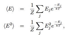
The Partition function is also a generating function for the Thermodynamic variables like the average internal Energy (U) of the system:

and the Helmholtz Free Energy (
And if we minimize the Free Energy (ala Hinton), the resulting probabilities follow the Boltzmann / Gibbs Distribution.
We don’t frequently see use the all of the machinery statistical mechanics in Deep Learning. In particular,
in ML, the Temperature is set implicitly to 1

Note that T is not 0. Methods that minimize the Free Energy, or at least operate at T=1, are effectively averaging over the minima T=0 landscape–they smooth out the non-convexity.
Convex and non-Convex Optimization
In simpler machine learning algos like SVMs and Logistic Regression, we can readily solve the optimization problems using Stochastic Gradient Descent (SGD)– because these are convex optimization problems.
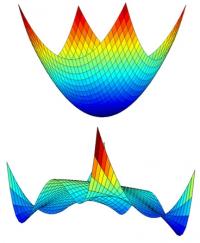
Below we see two optimization surfaces: our goal is to find the global minimum. The top problem is easy to solve, and just about any decent descent method will do (unless we need sparse solutions, which makes this a little trickier). The bottom problem, however, is filled with hills and bumps, and even looking at it, we are not sure where the bottom is.
So how do we find it? Typical solvers for non-convex problems include Genetic Algorithms, Convex-Concave/DC programming, BackProp (for ANNs), and Simulated Annealing. 
In Simulated Annealing, we run the solver until it gets stuck. We then heat the system, making it jump over local humps. We then cool it down–we run the solver again until it stops. We repeat this over and over until we find the global minimum. A common application is in the simulation of liquids and crystals. To do this, we need to define a temperature.
However, not every method is just seeking a global minima.
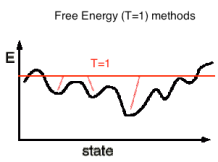
Free Energy methods, operating at (T>0), effectively sample all the low lying local minima simultaneously.
Statistical mechanics allows us to add a Temperature to our probabilistic modeling methods and the define Free Energy through the framework of the Canonical Ensemble.
Adding Temperature to Probabilistic Modeling
In traditional probability theory, we require the individual probabilities sum to 1:

Of course this is always true, but we don’t have to enforce this all the time; we can relax this constraint and simply enforce it at the end of the problem. This is exactly what we do in Simulate Annealing. Instead of creating probability models, we create Energy Models. The energies are essentially the log of unnormalized probabilities

We only require the total energy 


we need the normalization factor


Modeling with Energies
Lets say we have a bunch of objects that we would like to distribute (or cluster) into boxes, sets, or sequences in some optimal way. We might be placing balls into boxes, or we could be assigning documents into clusters, or considering the activated neurons in a network. We want to find the optimal way of doing this through some constrained optimization problem. Imagine we have a container partitioned into small, disjoint boxes or sets 

- the total number of objects $latex \mathcal{N} $ is fixed. For us, the total number songs.
- the total ‘Volume’ V is fixed. This will come up later when we create the metric embedding
We seek the probability 


Each combination, or set of numbers, 


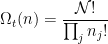
Each combination has a specific configuration of energies 
![]() the total energy of this configuration (or micro-state) is given by
the total energy of this configuration (or micro-state) is given by
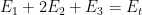
irrespective of the explicit ordering. We can consider other configurations as well
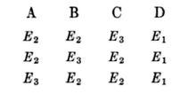
but they all have the same total energy 
The probabilities of being in each box 

where 


We want to find the most likely distribution 


as is the most likely average Energy
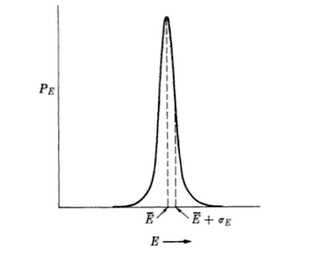
Which means that we can approximate the most likely distribution by trying to find the minimum value of


We can solve this optimization using the method of Lagrange multiplies, as we do in many convex optimization problems in ML. This yields
![\dfrac{\partial}{\partial n_{j}}\left[\ln\Omega_{t}(n)-\alpha\sum_{i}n_{i}-\beta\sum_{i}n_{i}E_{i}\right]=0](https://s0.wp.com/latex.php?latex=%5Cdfrac%7B%5Cpartial%7D%7B%5Cpartial+n_%7Bj%7D%7D%5Cleft%5B%5Cln%5COmega_%7Bt%7D%28n%29-%5Calpha%5Csum_%7Bi%7Dn_%7Bi%7D-%5Cbeta%5Csum_%7Bi%7Dn_%7Bi%7DE_%7Bi%7D%5Cright%5D%3D0+&bg=ffffff&fg=%23000000&s=0&c=20201002)
where 

Stirling’s Approximation

to write

Now we can evaluate the derivatives explicitly

With this simple expression, we can find the optimized, average number of objects in each box

where

and the optimal probability of being in each box
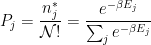
which is known as as the Boltzman Distribution, or , more generally, the Gibbs Measure.
The average energy of the system, which is a kind of optimal normalization for the problem, is given by

We now recognize that the energies are log probabilities
and we call the normalization factor the Partition Function


We call 

Temperature as Energy Fluctuations
The Temperature is related to Energy Fluctuations in the Canonical Ensemble. We can write:
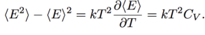
where Cv is the system heat capacity, and we define the equilibrium fluctuations as
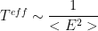
The Temperature sets the scale of the Energy. We note that in many neural networks and inference problems, we implicitly T=1. We sometimes call this being scale-free.
In the T=1 case, however, if we actually try to measure true, the effective Temperature, we would find that it scales inversely with the empirical Energy fluctuations
We also would find that, as the system size N increases, the Energy fluctuations should become negligible.
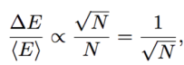
This is actually violated near a phase transition, leading to the following…
Caveats:
The Boltzmann Distribution only arises in weakly interacting systems, where this decomposition / energy partitioning actually applies. At least the Energy should be extensive and the Thermodynamic limit should exist. But this is not all.
In strongly interacting systems–such as near a phase transistion–we need specialized techniques. Onsager solved this problem for the 2D Ising Model. More generally, Renormalization Group techniques may be needed.
Summary
We have completed out mission; we have introduced the notion of a Temperature into our probabilistic models and deriving the Canonical ensemble.
Still, we see that the language of Statistical Physics offers many advantages over traditional probabilistic models–and this why it is so popular in machine learning.

It’s a very interesting post, it is always nice to see the fundamental principles of the methods we often use in ML (and sometimes forget what stands behind them). However, I find a few points difficult to digest. Could you shed some light on them?
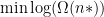
1. I see you are looking for the most likely arrangement of the ‘balls’ in the boxes. But what allows you to switch from searching for the maximum likelihood to the minimum one? I refer to the $\min \log \Omega(n)$.
2. I don’t see the argument connecting logarithmic function with the ‘peakiness’ of the distribution. I have always been thinking that the the reason of the log-mapping stem from the monotonicity preservation of log for certain family of the logarithmic basis.
3. I would be interested in understanding why by increasing T (or decreasing the Lagrange multiplier) we enable the optimizer to ‘jump’ over the local minima. What is the algebraic argument? Is it somehow connected with the Stochastic Gradient Methods?
Thanks!
LikeLike
1. by the most likely arrangement i mean the one that is most probable. what is ‘the minimum one’?
2. because the distribution is highly peaked, when we take the log, the distribution does not really change that much. this was the classical argument; these days people kinda ignore this point and just assume that the log of the distribution is representative of the distribution, and that’s not the case in the tails of the distribution for small data sets
3. Yeah we don’t really adjust T in the SGD itself. What we do is take a random jump, and then accept or reject the jump based on temperature threshold. I need to explain in code so i will try to write some up.
what language is best? ruby? python? java? lua?
Thanks for the comments…its very helpful to have some feedback
LikeLike
on 1. I might have switched a sign let me check and get back to you
on 2. yes this is subtle but it is the intent. this is sometimes missed in ML
on 3. SGD only works for convex methods…
LikeLike
Hi, I was thinking of aggregating your posts into a toolkit (python perhaps?), do you think it would be useful?
LikeLike
we could certainly do something like this with some of the newer posts
I have a lot of ideas and not enough time to write up everything
usually I make a github account and post code there, as i did with the ruby work
I had some issues displaying the ipython notbook on wordpress and it is was unclear to me if i need to upgrade to a paid account to do this
do you know?
LikeLike
Hi, have you seen this post: http://www.josephhardinee.com/blog/?p=46 ?
LikeLike
yes this is for self-hosted wordpress where you can modify the css directly
it was unclear to me if histed wordpress would allow this
LikeLike