Rethinking–or Remembering–Generalization in Neural Networks

I just got back from ICLR 2019 and presented 2 posters, (and Michael gave a great talk!) at the Theoretical Physics Workshop on AI. To my amazement, some people still think that VC theory applies to Deep Learning, and that it is surprising that Deep Nets can overfit randomly labeled data. What’s the story ? Let me share an updated version of my thoughts on this.

Last year, ICLR 2017, a very interesting paper came out of Google claiming that

Understanding Deep Learning Requires Rethinking Generalization

Which basically asks, why doesn’t VC theory apply to Deep Learning ?

In response, Michael Mahoney, of UC Berkeley, and I, published a response that says

Rethinking generalization requires revisiting old ideas [from] statistical mechanics …

In this post, I discuss part of the motivation for our paper.

Towards a Theory of Learning

In the traditional theory of supervised machine learning (i.e. VC, PAC), we try to understand what are the sufficient conditions for an algorithm to learn. To that end, we seek some mathematical guarantees that we can learn, even in the worst possible cases.

What is the worst possible scenario ? That we learn patterns in random noise, of course.

Theoretical Analysis: A Practical Example

“In theory, theory and practice are the same. In practice, they are different.”

The Google paper analyzes the Rademacher complexity of a neural network. What is this and why is it relevant ? The Rademacher complexity measures how much a model fits random noise in the data. Let me provide a practical way of thinking about this:

Imagine someone gives you $m$ training examples, labeled data $\mathbf{X},\mathbf{y}$ , and asks you to build a simple model. How can you know the data is not corrupted ?

If you can build a simple model that is pretty accurate on a hold out set, you may think you are good. Are you sure ? A very simple test is to just randomize all the labels, and retrain the model. The hold out results should be no better than random, or something is very wrong.

Our practical example is a variant of this:

Build a simple model. Like a linear SVM. Then optimize. Let’s say we get 95% training accuracy, and 90% test (generalization) accuracy, and that this is pretty good.
Randomize some of the labels in the training data. Like %10. Of course, you may overtrain now. So optimize again. That means adjust the regularization. Repeat this many times (i.e. 100x). Find the worst possible training and generalization accuracies.

By regularizing the model, we expect we can decrease the model capacity, and avoid overtraining. So what can happen ?

easy case If the data is really clean, and since first model (1) is pretty good, we might expect then the worst training accuracy (2) should be about ~10% less than the first. After all, how could you as generalize well if you added noise to the data ?! So we might find that, for (2) , a training accuracy of 85%, and generalization accuracy of 90%.
hard case The worst training accuracy (2) remains at 95%. And the generalization accuracy stays around 80% or so. You randomized 10% of the labels and nothing really changed ?! Are you just overtraining ? Or are the labels corrupted ?
- Remember, we picked a very simple linear SVM. it has 1 adjustable parameter —the regularization parameter. And maybe that did not even change much. And if you overtrained, the training error would be zero, and the generalization error much larger.
- So chances are, the data is corrupted. and you were asked to build good model using very noisy data. Been there, and it is no fun.

Notice in both cases, the difference in training error $e_{t}$ and generalization error $e_{g}$ stayed nearly fixed or at least bounded

$|e_{g}-e_{t}|\leq 5\%$

pathological case The Google paper claims: “Even with dropout and weight decay, Inception V3 is still able to fit [a] random training set extremely well if not perfectly.” But the generalization accuracy tanks. (See Table 2):

$|e_{g}-e_{t}|\rightarrow 100\%$

It appears that some deep nets can fit any data set, no matter what the labels ? Even with standard regularization. But computational learning theories, like VC and PAC theory, suggests that there should be some regularization scheme that decreases the capacity of the model, and prevent overtraining.

So how the heck do Deep Nets generalize so incredibly well ?! This is the puzzle.

The Effective VC Dimension of a Neural Network: Vapnik and LeCun

Before we dive in Statistical Mechanics, I first mention an old paper by Vapnik, Levin and LeCun, Measuring the VC Dimension of a Learning Machine (1994) .

It is well known that the VC bounds are so loose to be of no practical use. However, it is possible to measure an effective VC dimension–for linear classifiers. Just measure the maximal difference in the error while increasing size of the data, and fit it to a reasonable function. In fact, this effective VC dim appears to be universal in many cases. But…[paraphrasing the last paragraph of the conclusion]…

“The extension of this work to multilayer networks faces [many] difficulties..the existing learning algorithms can not be viewed as minimizing the empirical risk over the entire set of functions implementable by the network…[because] it is likely…the search will be confined to a subset of [these] functions…The capacity of this set can be much lower than the capacity of the whole set…[and] may change with the number of observations. This may require a theory that considers the notion of a non-constant capacity with an ‘active’ subset of functions”

So even Vapnik himself suspected, way back in 1994, that his own theory did not directly apply to Neural Networks!

What changes people’s minds ? They started to realize that the Loss functions (and Energy Landscapes E[(W,b)]) in DNNs might actually be convex. But this was also known in the late 90s

Here’s the thing–just because the problem looks convex locally does not imply it is complex globally. That is, the Energy Landscape and./or the Loss looks convex locally, in Vapnik’s subset of functions. So being an old man, I was not really surprised.

Since we are reaching into the past…what does the old physics have to say ?

Statistical Mechanics:

In physics, VC theory is just a 1 page appendix in a 300 page book on the Statistical Mechanics of Learning. But don’t read all that–let me give you the executive summary:

The Thermodynamic Limit

We argue that the whole idea of looking at worst-case-bounds is at odds with what we actually do in practice because we take a effectively consider a different limit than just fixing m and letting N grow (or vice versa).

Very rarely would we just add more data (m) to a Deep network. Instead, we usually increase the size of the net (N) as well, because we know that we can capture more detailed features / information from the data. So, win practice, we increase m and N simultaneously.

In Statistical Mechanics, we also consider the join limit $m,N\rightarrow\infty$ …but with the ratio m/N fixed.

The 2 ideas are not completely incompatible, however. In fact, Engle… give nice example of applying the VC Bounds, in a Thermodynamic Limit, to a model problem.

Typical behaviors and Phase Behavior

In contrast to VC/PAC theories, which seek to bound the worst case of a model, Statistical Mechanics tries to describes the typical behavior of a model exactly. But typical does not just mean the most probable. We require that atypical cases be made arbitrarily small — in the Thermodynamic limit.

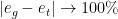
This works because the probabilities distributions of relevant thermodynamic quantities, such as the most likely average Energy, become sharply peaked around their maximal values.

Many results are well known in the Statistical Mechanics of Learning. The analysis is significantly more complicated but the results lead to a much richer structure that explains many phenomena in deep learning.

In particular, it is known that many bounds from statistics become either trivial or do not apply to non-smooth probability distributions, or when the variables take on discrete values. With neural networks, non-trivial behavior arises because of discontinuities (in the activation functions), leading to phase transitions (which arise in the thermodynamic limit).

3 phases of learning

For a typical neural network, can identify 3 phases of the system, controlled by the load parameter $\alpha=\dfrac{m}{N}$ , the amount of training data m, relative to the number of adjustable network parameters N (and ignoring other knobs)

Memorization: $\alpha$ very small.
Overtraining: $\alpha$ too small
Generalization $\alpha$ large

Now maybe the whole issue is just that Deep Nets have such a massive capacity that they are just memorizing ( $\alpha$ is very small).

Generally speaking, memorization is akin to prototype learning, where only a single example is needed to describe each class of data. This arises in certain simple text classification problems, which can then be solved using Convex NMF (see my earlier blog post).

Maybe DNNs are memorizing ? But let suggest an alternative:

What is Over Training ?

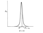
In SLT, over-training is a completely different phase of the system, characterized by a kind of pathological non-convexity–an infinite number of (degenerate) local minimum, separated by infinitely high barriers. This is the so-called (mean field) Spin-Glass phase.

SLT Overtraining / Spin Glass Phase has an infinite number of deep minima

So why would this correspond to random labellings of the data ? Imagine we have a binary classifier, and we randomize $L$ labels. This gives $2^{L}$ new possible labellings:

Different Randomized Labeling of the Original Training Data

We argue in our paper, that this decreases the effective load $\alpha$ . If $L\ll N$ is very small, then $\alpha$ will not change much, and we stay in the Generalization phase. But if $L\sim\mathcal{O}(N)$ is of order N (say 10%), then $\alpha$ may decrease enough to push us into the Overtraining phase.

Each Randomized Labelling corresponds to a different , deep, (nearly) degenerate minima on the global Energy Landscape E_DNN([W,b])

Moreover, we now have $2^{L}$ new, possibly unsatisfiable, classifications problems.

Of course, each problem has a different loss function…so they naively look like different problems. But all of these solutions produce a final, trained neural network with a shared, final Energy Landscape E_DNN([W,b]), defined solely by the final weights and biases learning in training.

So the final Energy Landscape will be nearly degenerate. But many of these will be difficult to learn because the many of label(s) are wrong, so the solutions could have high Energy barriers — i.e. they are difficult to find, and hard to get out of.

So we postulate by randomizing a large fraction of our labels, we push the system into the Overtraining / Spin Glass phase–and this is why traditional VC style regularization can not work–it can not bring us out of this phase. At least, that’s the theory.

—

To learn even more about this, see the great book by Engle and Van der Broeck, the Statistical Mechanics of Learning.