Eigenvalue-Independent Effective (Semantic) Operator

This post is still just sketch of ideas…not ready for consumption

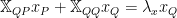
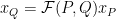
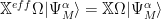
In my last post I introduced the Eigenvalue-Dependent Effective (Semantic) Operator as a Semantic Similarity metric that couples visible (P) and hidden (Q) features:

$\mathbb{X}^{eff}(\lambda)= \mathbb{X_{\mathrm{PP}}}+\mathbb{X_{\mathrm{PQ}}}(\lambda_{x}-\mathbb{X}_{QQ})^{-1}\mathbb{X_{\mathrm{QP}}}$

where $\mathbb{X}$ is the complete feature-feature coupling matrix (such as a giant TFIDF matrix for all the term, tags, and other features in a large document collection) and $\lambda$ is the dominant eigenvalue of $\mathbb{X}$ .

$\mathbb{X}^{eff}(\lambda)$ is useful for dimensional reduction when the hidden dimensions are actually useful and not just noise.

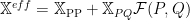
It is necessary, however, to solve find the dominant eigenvalue of $\mathbb{X}$ . In some cases, however, it may be quite hard to find this eigenvalue. In other cases, we may want to de-noise or regularize the hidden variables. Or perhaps there is clearly more than just one dominate eigenvalue? What can we do?

We now introduce the Eigenvalue-Independent Effective (Semantic) Operator , using techniques from quantum mechanical many body perturbation theory (MBPT), that resolves all of these issues.

The Correlation Operator

Consider again the eigenvalue equation for the feature correlation matrix $\mathbb{X}$

$[\begin{array}{cc} P\mathbb{X}P & P\mathbb{X}Q\\ Q\mathbb{X}P & Q\mathbb{X}Q \end{array}]\begin{array}{c} Px\\ Qx \end{array}= \lambda\begin{array}{c} Px\\ Qx \end{array}$

We now re-write this using subscripts, and identify the expressions for the P and Q space

$\mathbb{X_{\mathrm{PP}}}x_{P} +\mathbb{X}_{PQ}x_{Q}= \lambda_{x}x_{P}$ Visible Space (2)

$\mathbb{X}_{QP}x_{P}+\mathbb{X}_{QQ}x_{Q}=\lambda_{x}x_{Q}$ Hidden Space (3)

Recall before we formed an explicit expression for $x_{Q} (\lambda)$ from equation (3) , so that

$x_{Q}(\lambda) = (\lambda_{x}-\mathbb{X}_{QQ})^{-1}\mathbb{X}_{QP}x_{P}$

Fet us define a new operator, $\mathcal{F}(P,Q)$ , called the Correlation Operator, that explains how our hidden features to our visible features:

$x_{Q}=\mathcal{F}(P,Q)x_{P}$

Our goal can be restated as to find a suitable Correlation Operator $\mathcal{F}(P,Q)$ that does not depend on $\lambda$ and yet generates the Effective Operator we seek. What does this mean? Lets plug $\mathcal{F}(P,Q)$ backing into equations (2) and (3) and find a (non-linear) relationship between the equations, subject to the constraints that the Effective Operator be Hermetian and span the entire P-space (i.e. includes all tags). [Below we refer to this as a Complete Model Space of features ]

$\mathbb{X_{\mathrm{PP}}}x_{P} +\mathbb{X}_{PQ}\mathcal{F}(P,Q)= \lambda_{x}x_{P}$ Visible Space (4)

$\mathbb{X}_{QP}x_{P}+\mathbb{X}_{QQ}\mathcal{F}(P,Q)=\lambda_{x}\mathcal{F}(P,Q)x_{P}$ Hidden Space (5)

using the definition of $latex \mathcal{F}(P,Q) $, multiply the R.H.S. of (4) by this to obtain

$\mathcal{F}(P,Q)\mathbb{X_{\mathrm{PP}}}x_{P} +\mathcal{F}(P,Q)\mathbb{X}_{PQ}\mathcal{F}(P,Q)= \lambda_{x}\mathcal{F}(P,Q)x_{P}$ Visible Space (6)

Subtracting equation (5) and (6) to into a single equation

$\mathbb{X}_{QP}x_{P}+\mathbb{X}_{QQ}\mathcal{F}(P,Q)-\mathcal{F}(P,Q)\mathbb{X_{\mathrm{PP}}}x_{P} -\mathcal{F}(P,Q)\mathbb{X}_{PQ}\mathcal{F}(P,Q) =0$ (7)

Our goal is then to find $\mathcal{F}(P,Q)$ that satisfies (7) for every eigenvector in the primary space P simultaneously. There are many ways to do this in the chemical physics literature; here I will explain the ones I believe that may have application in Machine Learning.

In particular, we do not seek an exact Effective Operator since , usually in Machine Learning, our input data is noisy and may only have a few significant figures. Indeed, we expect that an approximate Effective Operator will perform better than the exact solution. Also, we may want to add a regularizer, and we will need a formalism that permits this.

Our Effective Operator will take the form

$\mathbb{X}^{eff}=\mathbb{X_{\mathrm{PP}}}+\mathbb{X}_{PQ}\mathcal{F}(P,Q)$

but this operator may not be Hermertian– a requirement for a Machine Learning Kernel. We can, however, in certain cases, form the associated Hermetian effective operator by taking the sum of $\mathbb{X}^{eff}$ and it’s Hermetian conjugate — a process we call Symmetrizing the Operator

$\mathbb{X}^{eff}_{sym}=\frac{1}{2}\{\mathbb{X}+(\mathbb{X}^{eff})^{*}\} =\mathbb{X_{\mathrm{PP}}}+\frac{1}{2}\{\mathbb{X}_{PQ}\mathcal{F}(P,Q)+\mathcal{F}^{*}(P,Q)\mathbb{X}_{PQ}\}$

Finally, we are not really trying to model an eigenvalue problem but rather the (semantic) feature-feature similarities. Consequently, we will need a formalism that lets us treats features explicitly, and does not just model the eigenvalues and eigenvectors of $\mathbb{X}$ . In the language of Effective Operators, this means the Primary Space must be a Complete Model Space.

So how do we get here? While the final result is quite simple, the road to get there is long and technical.

Notation: Primitive Features and Hilbert Spaces

Lower case letters (p) refers to primitive features like tags $\tau$ , words, etc.

We refer to the space of features $\mathcal{F}$ as the complete set of all features

$\mathcal{F {f|f\epsilon\mathcal{F}\}$

In physics and chemistry, $\mathcal{F}$ is the Fock Space.

The spaces $\mathcal{P},\mathcal{Q}$ are Hilbert spaces, spanned documents, instances, and general vectors x, $latex \Psi $, etc. These vectors are linear combination of primitive features $x=\sum w_{p}|p\rangle+\sum w_{q}|q\rangle$

Identifying Primary Features

Let us consider in more detail how we define our features spaces $P,Q$ and the feature correlation matrix $\mathbb{X}$ . How can we know we can partition our features into $P,Q$ ? We can do this when the the P-space features $|p\rangle$ , such as the tags $\tau$ , dominate the principle eigenvectors of $\mathbb{X}$ . That is, for the dominant eigenvector

$x_{0}=\sum w_{p}|p\rangle+\sum w_{q}|q\rangle$

the p-space weights $latex w_{p} $ are much larger than the q-space weights $w_{q}$

$latex w_{p}\gg w_{q} $

More importantly, lets consider how the Eigenvalues of $\mathbb{X}$ are distributed.:

Here I sketch the possible eigenvalues of the feature density matrix $\mathbb{X}$ ; you can also think of these as the singular values arising from an SVD/LSA like calculation. First, note that we expect the largest eigenvalues to correspond to eigenvectors that are dominated by the P-space features (p), and we refer to these as the P-space eigenvalues. Ideally, we might hope that we can identify a complete set of high lying eigenvectors that are totally dominated by the P-space features. That is, t if we were to run SVD/LSA, then we expect that lowest clusters / singular vectors would be dominated by P-space features. Typically, however, we may observe that only the few largest eigenvalues as dominated by P-space features (and the smallest by Q-space features), whereas the mid-range eigenvectors are harder to classify. Hence the need for a simple model.

It is precisely this distinction among features — the ability to identify a dominate class of features — that allows us to apply the Effective Operator technique. In some cases, this will be self-evident. In others, it might seem fictitious since we decided beforehand how to construct the feature density matrix $\mathbb{X}$ . I will address various examples in a future post–for now, I would like to get the basic mathematical result.

The Complete Model / Feature Space

Let’s consider how we might identify a model space $\mathcal{P}_{M}$ of primary features (like tags). Since we expect the most important P-space eigenvectors $x_{p}$ to be dominated by p-space features, we have

$|x_{p}\rangle =\sum w_{p}|p\rangle + \cdots$

We do not know yet what the P-space actually is. We might try to pick it using an SVD/LSA approach–we simply pick the N lowest eigenvectors of $\mathbb{X}$ . But we could not use this to compute a Semantic similarity $\langle \tau'|\mathbb{X}^{eff}|\tau \rangle$ . We must be able to express $latex \mathbb{X}^{eff} $ in a basis of the original P-space features:

$\mathbb{X}^{eff}=\sum_{p,p'}|p\rangle\mathbb{X}_{p,p'}^{eff}\langle p|$

Since we don’t know it, we will guess. We model the true P-space eigenfunctions by the space of functions $\mathcal{P}_{M}$ that is isomorphic the P-space sublock of the feature density matrix, $P^{t}\mathbb{X}P$ , such that

$latex \mathcal{P}_{M}\sim P^{t}\mathbb{X}P $

We write the model primary and secondary space projection operators as

${P}_{M}=\sum_{p,p'}|p\rangle\ \langle p|$ and

$Q_{M}=\sum_{q,q'}|q\rangle\ \langle q|$

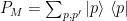
We call the model space $\mathcal{P}_{M}$ a Complete Model Space because it is spanned only by the p-space features. Notice this is space (while isomorphic to) is quite different from the P-space we might obtain from taking the first $N_{P}$ eigenfunctions of $\mathbb{X}^{eff}$ because these latter functions have non-zero Q-space features weights.

Indeed, we are , in the most literal sense, constructing a Model for our problem, and seeking to describe the true situation with this highly accurate, de-noised, interpretable and explainable model.

The Wave Operator and the Generalized Bloch Equation

How do we relate our Model Space back to actual data clusters? We have measured the correlations between our features and formed the matrix $\mathbb{X}$ . We wish to model the major clusters of our data, which, in our approach, is the same as modeling the top $N_{P}$ , target eigenfunctions of $\mathbb{X}$

$\mathbb{X}|\Psi^{\alpha}\rangle=\lambda^{\alpha}|\Psi^{\alpha}\rangle$ where $\alpha=1...N_{P}$

We assume there exists a operator $\Omega$ , called the Wave Operator, that relates our model functions $|\Psi_{M}^{\alpha}\rangle$ to our original target eigenfunctions, as

$|\Psi^{\alpha}\rangle=\Omega|\Psi_{M}^{\alpha}\rangle$ for all $\alpha=1...N_{P}$

Moreover, we seek to model the semantic similarity between the model features

We therefore need a way to relate the Wave Operator to our Effective (Semantic Similarity) Operator; we will achieve this via the Generalized Bloch Equation

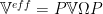
We define the Effective Operator as an operator that acts on the model space functions and generates the associated eigenvalues of the feature-feature correlation matrix $\mathbb{X}$

$\mathbb{X}^{eff}|\Psi_{M}^{\alpha}\rangle =\lambda^{\alpha}\Psi_{M}^{\alpha}\rangle$ for all $\alpha=1...N_{P}$

If multiply both sides of this by $ \Omega $ , we obtain

$\Omega \mathbb{X}^{eff}|\Psi_{M}^{\alpha}\rangle =\lambda^{\alpha}|\Psi^{\alpha}\rangle$

We can also insert $\Omega$ into our original eigenvalue problem, to give

$\mathbb{X}\Omega|\Psi_{M}^{\alpha}\rangle =\lambda^{\alpha}|\Psi^{\alpha}\rangle$

We can combine these equations as

$\mathbb{X}^{eff}\Omega|\Psi_{M}^{\alpha}\rangle =\mathbb{X}\Omega|\Psi_{M}^{\alpha}\rangle$ for all $\alpha=1...N_{P}$

Since this expression holds for all model space functions (for all $\alpha$ ), this leads to

The Generalized Bloch Equation

$\mathbb{X}^{eff}\Omega P =\mathbb{X}\Omega P$

But we need one more constraint or relation to obtain the complete for our Effective Operator. And we have it. We apply what is called

Intermediate Normalization

We require that our model functions and our actual functions overlap, and we set this overlap to one

$1$ for all $\alpha=1...N_{P}$

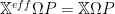
If we multiply P to the R.H.S. of the Generalized Bloch Equation, we obtain our final expression:

$\mathbb{X}^{eff}=P\mathbb{X}\Omega P$

We now need a way to compute the Effective Operator…which brings us to

Many Body Perturbation Theory

As with many numerical matrix methods, to solve our Effective Operator equation, we decompose $\mathbb{X}$ into two parts

$\mathbb{X}=\mathbb{U}+\mathbb{V}$

For example, in many method, $\mathbb{U}$ is the diagonal part of $\mathbb{X}$ . For later purposes, we shall choose a form such that $\mathbb{U}$ may be generated directly from the individual features as a sum of matrix expressions $u_{p,p'}, u_{p,q'}, u_{q,q'}$ :

$\mathbb{U}=\sum_{p,p'}|p\rangle u_{p,p'}\langle p'|+\sum_{p,q'}|p\rangle u_{p,q}\langle q|+\sum_{q,q'}|q\rangle u_{q,q'}\langle q'|$

We will chose a partitioning that reflects both our physical knowledge of the system and our noise. In particular, we will assume $\mathbb{V}$ carries the noise, and therefore we only include a small piece of $\mathbb{V}$ .

Indeed, rather than Regularize, which is the standard Machine Learning approach, we will assume that we can treat the noise using low-order perturbation theory, and 1 or more adjustable parameters.

We can now re-write the Effective Operator in Partitioned Form

$\mathbb{X}^{eff}=P\mathbb{U}P+P\mathbb{V}\Omega P$

We can also directly express

$\mathbb{V}^{eff}=P\mathbb{V}\Omega P$ and

the Partitioned Form of the Generalized Bloch Equation

$(\Omega\mathbb{X}^{eff}-\mathbb{U}\Omega)P=\mathbb{V}\Omega P$

and, in terms of $\mathbb{V}^{eff}$

$(\Omega\mathbb{X}^{eff}-\mathbb{U}\Omega)P=Q(\mathbb{V}\Omega-\Omega\mathbb{V}^{eff})P$

We will now solve this equation using a low order Perturbation Theory.

Let us express $\Omega$ as a series expansion

$\Omega=I+\Omega_{1}+\Omega_{2}+\cdots$ ,

Since we only need a low order , approximate solution, we will form the so-called “second order” Effective Hamiltonian, which will take the form

$\mathbb{X}^{eff}=P\mathbb{X}P+P\mathbb{V}\Omega_{1} P$

We achieve this by forming an order-by-order expansion.

Let us assume, without loss of generality, that the P-space eigenvalues of $\mathbb{X}$ are degenerate with value $\lambda_{0}$ . This seems extreme, however, later we will justify this and explain how to correct for it at higher orders if necessary. We can re-write the Generalized Bloch Equation as

$latex (\lambda_{0}-\mathbb{U})\Omega P=Q\mathbb{V}\Omega P-\chi PV\Omega P $

where $\Omega=1+\chi$

We shall solve this by means of a Resolvent Operator.

Please stay tuned…this will take a while to finish….and to get the Latex formatting to work properly!

The Resolvent Operator Requires it’s own Blog Post so I will go do that first, then come back

“The aim of language…is to communicate…to impart to others the results one has obtained…As I talk, I reveal the situation…I reveal it to myself and to others in order to change it.” Jean-Paul Sartre