Dimensional Reduction via an Effective Operator

Introduction

Frequently in science, simple models work well beyond their expected range of accuracy and application, and can be essential to provide intuition and insight. Consquently, great effort goes into seaching for simple models that encompass only a few relevant variables and yet provide high accuracy, low bias, and good generalizability.

For example, in my former life as a Quantum Chemist, we constructed simple, semi-empirical models to predict the color of small pigment molecules.  The models were simple in that they were linear operators and that they explicitly treated only a small subset of the complete number of possible variables (i.e. only the  electrons).

http://pubs.acs.org/doi/abs/10.1021/jp960617w

These semi-empirical electron models embodied the best principals of modern modern machine learning techniques–they required only a small subset of data, generalized well to data never seen in the model, and effectively incorporated the biases of the problem in a general purpose formalism.  In fact, they are much, much simpler than solving the actual physical problem–the numerical solution of the many-electron quantum mechanical Schrödinger equation. The apparent success of semi-empirical quantum mechanical models sparked interest in our group at Chicago, and elsewhere, to develop a first principles, or ab initio, theory to explain why these models work so well. To the statistical machine learning (ML) community, this ab initio theory resembles a Kernel Dimensional Reduction method. Consquently, one wonders then if it is possible to develop a related, general purpose, Kernel Dimensional Reduction theory for machine learning, using some of the mathematical machinery of linear algebra and projection operators, and how this theory relates to existing formulations of ML.

In this post I will describe a new approach to Machine Learning and Feature Dimensional Reduction using what I call an Effective Regression Operator.  

Linear Regression

Consider the standard linear model for a regression (ala Smale: http://www.ams.org/notices/200305/fea-smale.pdf )

where is a vector of () features (or explanatory variables), is a set of () response variables (or dependent variables, or even labels), is a linear operator (i.e. a vector of weights), and is the error in our model. Furthermore, we assume only the dependent variables are subject to error, and the error is assumed to be come from normal random distribution with zero mean. Equivalently, we may say we are modeling the conditional expectation:

.

The machine learning/regression problem is to find that operator w that best statisfies our model. Typically this problem is over-determined; one takes a number of measurements (m), leading to a set of linear equations:

…

We may group these m equations together by grouping the measurement vectors () and the response vectors () into matrices, yielding the single linear equation

where y and e matrices (or vectors), w is an matrix , and is an matrix.

The goal is to find the optimal linear operator w which satisfies this equation.

Normal Equations 

To solve the problem, let us first rewrite the linear regression using the  normal equations :

 (1)

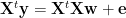
The common solution  (again, assuming normal errors) is the ordinary least squares (OLS) solution, found by constructing the Moore-Penrose Pseudoinverse of :

Regularization

Ridge Regression

Frequently the matrix is ill conditioned, so we may add a constant term (an adjustable parameter ) to the diagonal to regularize the solution, yielding:

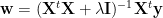
This is also known as Ridge regression. The regularization term  may be chosen using cross-validation. Equivalently (and more generally) the solution may be expressesed as a convex optimization problem:

Notice that, in general, the final model for should include terms from the null space of

Tikhonov Regularization

We may regularize the ill-conditioned inverse operator by adding an entire square matrix, as

This is called Tikhonov Regularization. We call the Tikhonov matrix, or, equivalently,   the Greens Function or Regularization Operator for the problem. This leads to the standard convex optimization problem seen in much of modern machine learning

We shall see that our Effective Operator takes the form of a  generalized Tikhonov Regularization.

Feature Partitioning: Visible and Hidden Variables

The fundamental assumption driving our approach is to explicitly partition the features into visible (P) and hidden (Q) features in order to explicitly reduce the dimensions of the problem

Let us partition our feature vector x into two subspaces (denoted P and Q), where the P subspace (the Primary space) contains features that are strongly correlated with the response variables, or labels,  y, and the other subspace Q (the Secondary space) contains those remaining features which are thereby weakly correlated to the labels y. That is, we choose the components such that is large, and such that is small.

We associate P with the visible features and Q with the hidden features

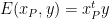
For each subspace P and Q, we identify the associated projection operators and , so that

As usual, the projections operators are idempotent:

  Visible Space

  Hidden Space

We denote the P and Q parts of the vectors using subscripts. For example, we write the primary features as and the secondary features as . Likewise, if is a matrix, we denote the action of projection operators with (upper case) subscripts, such as and . For consistency, we will never act on the left with the operators, thereby avoiding writing or .

We may now re-write above the normal equations (1) . First, for convenience, define

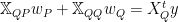
We may express this in block form as:

Now re-write this in block form (ignoring the error vector e) as

This leads to two seperate linear equations (using subscripts from now on)

  Visible Space (2)

  Hidden Space (3)

 Effective Regression Operator: :  

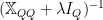
As a approximation, let us assume the hidden, Q-space variables are not coupled at all with the labels .  For example, if we don’t know the labels.  Then , yielding

This lets us write a simple expression for the hidden variable weight vector :

Substituting  for in equation  (2) above leads to a single, non-linear equation in the Visible P-space:

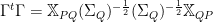
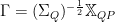
We now define the Effective Regression Operator :

 (4a)

where

(4b)

The Effective Operator acts only on the  Visible P space, and yet generates the exact solution to the orginal regression problem, subject to the Hidden-space approximation . (We may relax this approximation, shown below).

Generalizing Tikhonov Regularization

The Effective Regression Operator looks like a generalized Tikhonov regression, where the original regression is defined just over the P-space:

and where the Tikhonov matrix is given by

We may also write an formal expression for the Green’s Function .  Let us transform to a basis such that is diagonal. We have

yielding

We now see a simple interpretation of the Effective Operator   : it is a variance weighted coupling of the Visible P-space features to the Hidden Q-space features.

 In a later post we will also examine some real world examples and also see the  Fock Space / Second Quantization formulation.

Appendix

Series Expansion Approximation

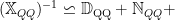
The term may be hard to compute if the Q-space is large and/or is hard to invert or perhaps ill-conditioned. Of course, we may add a regularization constant to the diagonal so that is well behaved.

It may not be enough to simply regularize the problem. Additionally, we will most likely need to regularize as well, so having two adjustable parameters may prove unwieldy.

We might hope to avoid a difficult matrix inversion by approximating using the matrix series expansion:

…

For example, let us split into a diagonal and non-diagonal matrices, such that:

and

so that

…

leading to simple expression to first order, with no matrix inverson necessary:

…

 Exact Effective Linear Regression: the Unbiased Solution

Let us now consider the general case of effective regression, where . Here, we derive an effective operator that acts on the P-space and gives the exact solution for the P-space weights

Within this formalism, one may then effectively de-noise the solution by creating approximations to and/or other parts of .

Going back to equation (3)

we write an exact expression for :

Plugging this expression for back into equation (2) this leads to a new regression problem

or, collecting terms, we get

This is significantly harder to solve because the effective equations are highly non-linear and the inverse operator appears on both sides of the equation.  I’ll leave the formal and numerical solutions and real world examples for a future post. [ We will also see how this relates to the Effective Operators that arise in Quantum Chemistry and Quantum Nuclear Physics. ]

Note:  I developed most of these ideas in 2001.  Subsequently, I have learned of some related approaches in the field of Gaussian Processes and Bayesian Regression that use the techniques of Hilbert Spaces and Projection Operators, such as  Huaiyu Zhu,  Christopher K. I. Williams,  Richard Rohwer & Michal Morciniec,  Gaussian Regression and Optimal Finite Dimensional Linear Models

One day I will sit down and try to determine the detailed relationship between these works.