Machine Learning with Missing Labels Part 3: Experiments

In this series of posts we look at Transductive and SemiSupervised Learning–an old problem, a hard problem, and a fundamental problem Machine Learning. Unlike Deep Learning or large scale ML,

We want to learn as much as we can from as labeled little data as possible.

We focus on text classification. Why?

The feature space is simple — its just words.
With the true labels, a simple SVM gives near perfect accuracy.
Text satisfies the cluster assumption.

Why isn’t this done all the time?

We can generate good (not great) Semi Supervised text classifiers. But

creating the input data is hard.
setting the input parameters is harder.
we can’t always distinguish the good solutions from the bad.

The 1st post looked at (1); here we try to understand (2&3), and look for simple, practical heuristics to make these old methods useful.

We can think of the TSVM/S3VM as generating several potentially good labelings on the unlabeled data. To solve (3), we need to find the best labeling–which means judging the label and/or classifier quality, such as the label entropy , cluster overlap, etc.

Or, alternatively, we might try to average the good solutions, similar to the way Hinton et. al. have recently suggested averaging an ensemble of models to take advantage of Dark Knowledge.

Thanks to Matt Wescott for pointing out this PDF and discussions on it.

To explore this, we run experiments using some old, existing, open source Transductive SVM (TSVM) and SemiSupervised SVM (S3VM) codes:

Our work is guided by the results in this 2014 paper on the QN-S3VM method, as applied to text data.

We thank Fabian Gieseke for help in reproducing and understanding these results.

For the TSVM, some available codes and algorithms are

SvmLight: Graph Cutting Algo
SvmLin: MultiSwitch (MS-TSVM) and Deterministic Annealing (DA-TSVM)
UniverSvm: Convex Concave Continuation Procedure (CCCP)
QN-S3VM: Quasi Newton SemiSupervised SVM

We can also compare the results to a SVM baseline, using either

LibLinear: various SVM and LR algos, or
Scikit-Learn SVC (Python Wrapper to LibLinear)

All these codes are Unix standalone C programs except QN-S3VM and Scikit-Learn, which are Python.

We examine SvmLin and its MultiSwitch (MS-TSVM) method.

SvmLin is the TSVM benchmark for most studies. After we work this up, we will move on to other codes listed. I also would like to test other TSVM/S3VM methods, such as S3VM-MIP, S4VM, S3VMpath, and many others, but may are MatLab codes and I don’t have C or Python open source code readily available. Or really the time 😛

We do not consider cases of weakly-supervised learning, where the labels may be both missing and/or have errors… but let me point out a 2013 paper on the WellSVM method. It also compares the above methods and is worth a read.

I hope this post gives some flavor to what is a very complicated and fundamental problem in machine learning. (And maybe take some ideas from Deep Learning to help solve the TSVM problem as well)

Methods: The real-sim Data Sets:

We care about text classification. To this end, we reproduce the performance of SvmLin, and, later, other methods, on the real-sim text dataset (listed in Table 2 in the paper). The real-sim dataset was used in the original SvmLin paper; it is an accepted baseline for these methods.

This data set consists of 72309 labeled documents: 22238 (+1) and 50071 (-1).

The fraction of positively labeled documents $R^{+}_{true}=30.75%$ .

Creating the Labeled, Unlabeled, and Holdout Sets:

I have created an IPython Notebook (make_realsim_inputs.ipynb) which can read the real-sim data and generate the input files for the various C programs listed above: SvmLight, SvmLin, & UniverSvm.

We can see it in the NBViewer here

The real-sim dataset is split in half, and 3 data sets are created. Half is used to train TSVM (labeled L and unlabeled U); the rest is a holdout set (HO) for testing.

Following Table 2, the notebook generates:

labeled (L) of sizes roughly: l=90, 180, 361, 1486, & 2892
an unlabeled set (U) of size u=36154-l.
a test or HoldOut set HO (of the remaining data)

Each data set (L,U,HO) also has ~0.31 fraction of labeled examples; U and HO are statistical replica’s of L, albeit larger.

The input files consist of a training file (or 2 files for SvmLin) and 3 test files (6 forSvmLin): labeled L, unlabeled U, and holdout HO. They are in the SvmLight format.

I.e. the SvmLin input files, for l=90, are:

filename size (lines) purpose

svmlin.train.90.examples 36154 labeled + unlabeled train tsvm

svmlin.train.90.labels 36154

svmlin.testL.90.examples 90 train labeled baseline

svmlin.testL.90.labels 90

svmlin.testU.90.examples 36154 evaluate unlabeled set

svmlin.testU.90.labels 36154

svmlin.testHO.90.examples 36155 evaluate holdout set

svmlin.testHO.90.labels 36155

Grid Searches with gnu parallel

Astoundingly, rather than performing a full grid search, many research papers fix the regularization parameters, guess them using some crude Bayesian scheme, or attempt to transfer them from some other data set. This makes it really hard to evaluate these methods.

We use a ruby script and the gnu_parallel program to run the command line unix programs and grid search the parameters. The script also computes the final HoldOut accuracy and metrics such as the margin and label entropy.

svmlin.rb

Gnu parallel lets us easily grid search the regularization parameters by running the TSVM codes in parallel.

We do a broad grid search

$W\in[.0001,0.001,0.01,0.1,1,10,100,1000,10000]$

$U\in[.0001,0.001,0.01,0.1,1,10,100,1000,10000]$

$R\in[0.25, 0.26, 0.27,\cdots,0.35,0.36,0.37]$

by creating a directory for each run

parallel "mkdir A2W{1}U{2}R{R}" ::: .0001 0.001 0.01 0.1 1 ::: 1 10 100 1000 1000 ::: 0.28 0.29 0.31 0.32 0.33 0.34

and then running SvmLin in each directory, simultaneously

parallel "cd A2W{1}U{2}R{R}; $SVMLIN -A 2 -W {1} -U {2} -R {3} ../svmlin.train.examples.90 ../svmlin.train.labels.90 > /dev/null" ::: 0.0001 0.001 0.01 0.1 1 ::: 1 10 100 1000 10000 ::: 0.28 0.29 0.31 0.32 0.33 0.34

We can then evaluate each run on the U or HO data set. We will find the optimal W and U are in the range of the original crude estimates W=0.001, U=1, and R=0.31

How can we evaluate the accuracy of our TSVM, here, and in a real world setting?

Ground Truth

Since we know the labels on both the U and the HO sets , these are a ground truth from which we can evaluate how well the best model(s) perform. We can get an upper bound on the best possible Generalization Accuracy (on the HO set) by training an SVM on L+U using the true labels, and then applying this model to HO.

The best expected HO accuracy here is ~ 97 %

Also, note this is different from the Reconstruction Accuracy on HO, which is > 99 %.

We might also obtain a better generalization accuracy with different features, such as applying GloVe or even unsupervised pre-training on L+U. We examine this in a future blog. We are, in particular, interesting in comparing the Deep Learning Auto-Encoders with Convex NMF, including recent variants applied to document clustering.

Baseline

We need a baseline for comparison. The IPython Notebook computes a baseline accuracy for the labeled data set (L); this can also be done with LibLinear or even SvmLin (using -A 1).

We then run the small L model on the HoldOut (HO) set for each l=90,180,…, yielding baseline accuracies of

split size	size of L (l)	HO Accuracy
0.0025	90	85 %
0.005	180	87.5 %
0.001	361	90 %
0.004	1446	93 %
0.008	2892	94 %

please note that these are computed from 1 random sample, and may be slightly different (by ~1%) for each run. Also, that the command line and scikit-learn liblinear have different defaults; we use C=10,fit_intercept=False.

Finding the Best Accuracy:

We are generating a large number of nearly equivalent models, parameterized by

$[\Gamma_{L}(U,W,R^{+})]$

The inputs are related to the objective function in blog post 1.

$W=\gamma$ , $U=\gamma'$ , and $r=0.31$

Every useful model will have the same reconstruction accuracy on the labeled examples L, and every model proposes a different soft labeling for the unlabeled examples U.

How can we compare different models $\Gamma_{L}(U,W,R^{+})$ ?

Essentially, we use a margin method to guess good labelings of the data, but we need an unsupervised heuristic to select the optimal labeling. Can we simply apply Cross-Validation to the small labeled set L? Or Leave One Out CV (LOO-CV) ? What filters can we apply to speed up the calculations ?

Best Accuracy on the Labeled Set

SvmLin may produce inferior or even nonsense models. But more subtly, some models may even have a very high training (on U), and a very high test accuracy (on HO), but a very low accuracy on L. These are not useful because in the real world, we don’t know the labels on U or HO.

We always want to first filter the possible solutions by selecting those with the best accuracy on the L.

Filter by Final Objective Function (FOF)

Since we are minimizing the objective function, we only consider solutions with FOF < 0.01. Note this is very different than simply assuming the best solutions has absolute minimum FOF across all input parameters.

We discard all solutions with Final Objective Function (FOF) > 0.01

For l=180, for example, this reduces the set of possible solutions from 1430 to 143.

Maximum Margin Solution…NOT

Wait, can’t we just take the solution with the maximum margin (or 1/norm)

$m=\dfrac{1}{\sum_{i}w_{i}^{2}}$

No. Think about how we practice supervised learning; we train a model, and set the regularization parameters by cross-validation. In the TSVM and SSL methods, we can can also apply CV (or LOO-CV), but only to the labeled set L.

The maximum margin solution is only best for a given set of input / regularization parameters (U,W,R). Every model $\Gamma_{L}(U,W,R^{+})$ induces a different labeling on U (that is, they form an equivalence class on L, not L+U). In fact, the best overall solution has the minimum margin amongst a broad scan of (U,W).

where the output weights $w_{i}$ are taken from

svmlin.training.examples.90.weights

Optimal Parameters for the HoldOut Test Accuracy

(this section is still under construction)

Cross Validation and Leave One Out on the Labeled Data

As with a standard SVM, one can try to apply Cross Validation (CV) to the labeled set L to select the best TSVM model. Most academic studies run 5-fold CV on the L set. This is harder, however, because

when L is small, the i.i.d. assumption fails, so CV my give spurious results
we really should use Leave One Out Cross Validation (LOO-CV), but this increases the run time significantly
the SvmLin code does not include CV or LOO-CV
the SvmLin DA-TSVM is unstable and I had to switch to MS-TSVM to complete this
my laptop cant take any more over clocking so I had to pause this for bit

I will finish this section once I either

modify SvmLin to run CV / LOO-CV
modify and use UniverSvm and the CCCP method, which is an order of magnitude faster than TSVM
and/or get this all working in IPython+Star Cluster so I can run LOO-CV at scale

Minimum Entropy of the Soft Labels

The SvmLin DA algo minimizes the entropy on unlabeled examples $S_{u}$ (it is the key stopping criteria, sec 3.2.3). Perhaps the model with minimum $S_{u}$ generalizes best?

This is the essence of Entropy Regularization--a common component of many Semi Supervised Learning formulations.

We can evaluate the proposed soft labels $\mu_{u}$ of the unlabeled set U, found in

svmlin.testU.examples.90.outputs

We convert soft labels to a probability $p_{u}$ :

$p_{u}=\dfrac{{\dfrac{{1}}{1+exp(-\mu_{u})}}}{\sum\dfrac{{1}}{1+exp(-\mu_{u})}}$

and compute the Entropy on U

$S_{u}=-\sum_{u}(p_{u}ln(p_{u})+(1-p_{u})ln(1-p_{u}))$

We hope that TSVM solutions with minimum $S_{u}$ will consistently yield a very good Generalization Accuracy (on the HO set) across a grid of search (U,W,R)–and preliminary results confirm this.

Let’s look at the l=90 case, and plot first the HO accuracy vs the Label Entropy $S_u$ .

Screen Shot 2014-10-31 at 8.38.15 PM

(Recall we only take solutions with FOF > 0.01 and the best training accuracy on the true labeled set.)

We see at 3-4 distinct sets of solutions with nearly equivalent entropy across a wide range of HO accuracy, and 2 classes include improved solutions (HO Accuracy > baseline 85%)

We call these Equivalence Classes under the Label Entropy.

Other solutions also show that the minimum Entropy solution is the best solution–for a fixed $R^{+}_{in}$ :

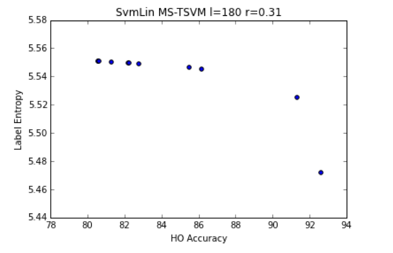
We select the minimum Entropy class of solutions.

Notice that the l=90 case is greatly improved above the 85% baseline, whereas l=1446 shows only a slight (0.5%) improvement–and 2-3% less than the best expected accuracy of 97%. We see the same results in the QN-S3VM and WellSVM papers, and suggests that

Transductive and SSL Learning may be limited to small labelled sets

where the percentage of labeled data is $L\sim 10-15%$ of U.

Predicted Fraction of Positive Examples

Recall we have to input an estimate $R^{+}_{in}$ of the fraction of positive labels on U $R^{+}_{U}$ .

We assume we estimate $R^{+}_{U}$ to within 10% using about 100 examples ( $l\sim O(100)$ )

We would prefer a high quality estimate if possible because the final, predicted $\hat{R}^{+}_{U}$ and $\hat{R}^{+}_{HO}$ appears to depend strongly on $R^{+}_{in}$ .

Here we test varying the input $R^{+}_{in}$ . We expect the predicted $\hat{R}^{+}_{HO}$ to be correlated with the generalization accuracies, and preliminary results also confirm this (note that all plots show the predicted fraction $\hat{R}^{+}_{HO}$ ):

Screen Shot 2014-10-31 at 8.38.48 PM

The predicted fraction $\hat{R}^{+}_{HO}$ also forms Equivalence Classes $\Gamma_{L,S}(R^{+})$ under the Entropy $S_{U}$ .

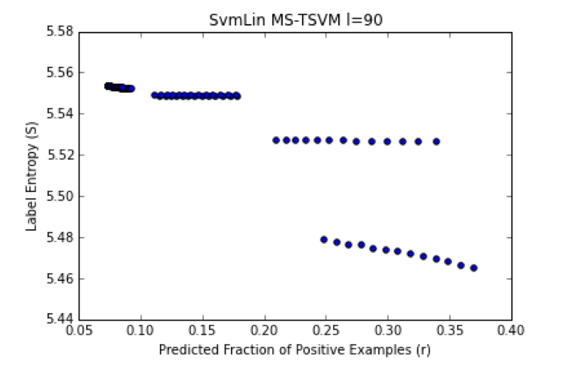
Of course, we know the true $R^{+}_{HO}=0.31$ , so the minimum Entropy solution is not the absolute best solution.

Perhaps a more generalized form of the Entropy would be more discerning? We would prefer a python toolbox like this one and need a way to fit the parameters.

We might also try to improve the TSVM search algorithm, as in the S4VM: Safe Semi-Supervised SVM methods. The S4VM tries to improve upon the SvmLin DA-TSM algo using Simulated Annealing, and then selects the best solutions by evaluating the final cluster quality. This looks promising for simple applications. Indeed, one might even try to implement it in python using the recent basinhopping library.

Transduction and the VC Theory

We have said that the VC Theory is a really theory about Transductive Learning.

We see now that to apply the TSVM in practice, the unlabeled data set U really needs to be an accurate statistical replica, as in the VC Statistical Learning Theory for Transduction.

We have tested cases where we have a good replica, but we did not estimate $R^{+}_{U}$ well; we have not yet tested cases where the U is NOT a good replica and we can only estimate $R^{+}_{U}$ partially. This needs to be done.

In the literature this is called using class proportions, and some recent estimatation methods have been proposed (and here)–although the QN-S3VM papers do not attempt this. Recently Belkin has shown how to estimate this fraction using methods of traditional integral methods.

The TSVM accuracy may depends on how well one can estimate the fraction (r) of positively labeled examples.

Also, we presume that TSVM models overtrain, and are biased towards either the (+) or (-) class.

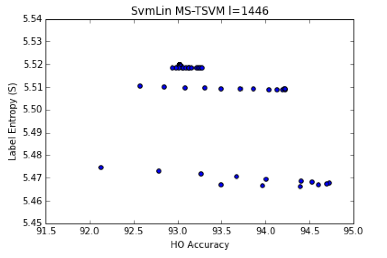
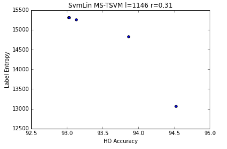
For l=1446, we find a single class of minimum Entropy entropy solutions

with $S\approxeq-5.467$ , W=0.001, U=1 and $\hat{R}^{+}_{HO}\in[0.25,0.37]$ .

They all have a high HO Accuracy–but may be biased towards choosing (+) labels because the minimum S solution has $\hat{R}^{+}_{HO}=0.36$ , not 0.31.

If we can’t estimate the $R^{+}_{U}$ well, may be able to average of the minimum Entropy solutions, thereby canceling out the biases in the over-trained models (i.e. average all $\hat{R}^{+}_{U}\in[0.28\cdots 0.34]$ TSVM models)

This is what Dark Knowledge, is all about–creating a simpler model by ensemble averaging– and we hope these recent advances in Deep Learning can help with Transductive Learning as well.

It is noted that the recent WellSVM method also addresses this problem. WellSVM uses a convex relaxation of the TSVM problem to obtain a min max optimization over the set of possible models allowed within a range of $R^{+}_{U}$ ; this is quite clever!

In a future blog, we will examine how the current TSVMs perform when tuning their parameters to obtain the best predicted fraction. If this is sound, in a future post, we will examine how to estimate the class proportions for text data.

Discussion

to come soon..stay tuned

Appendix

Each is TSVM is trained with a linear kernel. The regularization parameters are adjusted to give both optimal performance on the initial training set (L), and best reconstruction accuracy on the (U) set.

Each program requires slightly different command line options for these. There are also tuning parameters for each solver, and is necessary to set the tolerances low enough so the solvers can converge. For example, even for a linear SVM, the primal solvers may not converge as rapidly as the dual solver, and can even give different results on the same data set (despite Von Neumann’s minimax theorem). And the default for sckit-learn LinearSVC has the Bias on, whereas LibLinear has the Bias off. So be careful.

Below we show examples of training each the TSVMs on the labeled set (L), and evaluating the accuracy on a HoldOut set (HO), for l=90. We show typical values of the regularization parameters, but these do need to be tuned separately. We also show how to run the popular Liblinear program as a baseline (which uses the svmlight format); the paper uses LibSVM.

Baseline Linear SVM:

liblinear -C 0.1 -v 5 svmlight.testL.90

MS-SvmLin:

svmlin -A 2 -W 0.001 -U 1 -R 0.31 svmlin.train.examples.90 svmlight.train.labels.90

svmlin -f svmlin.train.examples.90.weights svmlight.testHO.examples.90 svmlight.testHO.labels.90

SvmLin DA:

svmlin -A 3 -W 0.001 -U 1 -R 0.31 svmlin.train.examples.90 svmlight.train.labels.90

svmlin -f svmlin.train.examples.90.weights svmlin.testHO.examples.90 svmlin.testHO.labels.90

SvmLight Graph Cuts:

svm_learn -p 0.31 svmlight.train.90 svmlight.model.90

svm_classify -C 100 svmlight.testHO.90 svmlight.model.90 svmlight.outHO.90

UniverSvm CCCP TSVM w/ramp loss:

universvm -C 1 -c 1 -s -0.5 -z 1 -o 1 -T universvm.testHO.90 universvm.train.90