Ever wonder what Google DeepMind is up to? They just released a paper on Semi-Supervised learning with Deep Generative Models. What is Semi Supervised Learning (SSL)? In this series of posts, we go back to basics and take a look.
Most machine learning algos require huge amounts of labeled data to achieve high accuracy. SVMs, Random Forests, and especially Deep Learning, can take advantage of massive labeled data sets.
How can we learn when we only have a few labeled examples?
In SSL, we try to improve our classifiers by taking advantage of unlabeled data.
In our last post we described an old-school approach to this problem, the Transductive SVM (TSVM), circa 2006. Here, we examine a different approach to learn from unlabeled data–Infernece with the Universum–ala Vapnik 2006.
Plus, there is code! The UniverSVM code has a TSVM and the Universum (USVM) approach.
Wait, doesn’t Deep Learning use unlabeled data in pretraining?
This is different. Deep Learning uses huge amounts of labelled data. We want to use as little labeled data as possible. To me, this is the real test of a learning theory.
In this and the next few blogs, we will examine at several variants of SVMs– USVM, WSVM, SVM+, and Semi Supervised Deep Learning methods–all that achieve high accuracy with only a small amount of labeled data. Also, we only consider text classification–images and other data sets require different methods.
Learning with Unlabeled Data
Let’s say with have a small number 

According to the Vapnik and Chervonenkis Statistical Learning Theory (VC-SLT), our generalization accuracy is very losely bounded by the model complexity and the number of training documents

which, in plain English, is just
Generalization Error 


The VC-SLT inspired the SVM maximum margin approach (although they are not equivalent).
SLT recognizes that for any data set 

![\Gamma_{L}=\left[\mathcal{H}_{1}\sim\mathcal{H}_{2}\sim\mathcal{H}_{3}\sim\cdots\right]](https://s0.wp.com/latex.php?latex=%5CGamma_%7BL%7D%3D%5Cleft%5B%5Cmathcal%7BH%7D_%7B1%7D%5Csim%5Cmathcal%7BH%7D_%7B2%7D%5Csim%5Cmathcal%7BH%7D_%7B3%7D%5Csim%5Ccdots%5Cright%5D+&bg=%23ffffff&fg=%23000000&s=0&c=20201002)
We should select the model 


This is easiest to visualize when the slack or admissible error = 1

Each model
The maximun margin is a measure of the VC capacity…
but is it the best?
While the VC-SLT bound is very loose, it does suggest that we usually need a large number of labeled documents
The SLT is, however, inherently a theory about Transductive Learning; the proof of the VC bounds requires first proving the Transduction bound (i.e. via Symmetrization). It has always been the dream of the VC-SLT program to develop a Transductive or SemiSupervised) method that can learn much faster than 
(By Semi-Supervised, we mean that the resulting model can be applied to out-of-sample-data directly, where as Transductive learning only applies to the known, unlabeled test set. We will not distinguish between them here.)
We would hope to achieve 
(Indeed, recently, Vapnik has shown it is actually possible to reduce this bound from 


If the max margin is the right measure, then the TSVM should work very well…
and yet, this has proved elusive.
What is the alternative ? Suppose instead of measuring the volume traced out by the hyperplanes, our models measured the volume between the convex hulls of the 2 classes:
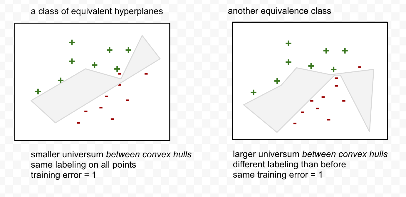
Notice that now, the labeling on the right is better.
This is a broader measure of the diversity of the equivalence class. In SLT, this is related to the VC Entropy (another measure of VC capacity).
The Universum approximates this volume–or rather the VC Entropy– via the Principle of Maximum Contradictions. (In fact, the Universum is not the only way to do this, as we shall see.) A clever idea–but something hard to achieve in practice. Let us compare and contrast the TSVM and the USVM to understand how to select the data sets they need and their limitations.
Transductive SVM (TSVM)
Transductive Inference requires a statistical replica 

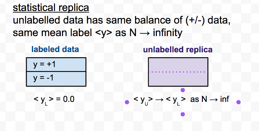
The replica 

In theory, we can always create a replica (or phantom sample) because we assume the labeled data itself is drawn from some common empirical process. In modern VC-SLT, we think of the symmetrization process that creates
In practice, we need to select the replica from unlabeled data–and this is hard!
We hope that by adding unlabeled data, we can find the best solution by guessing the labels of the unlabeled data and then maximizing the margin on all the data.

We can apply Transduction SVMs if we can create a large, unlabeled data set 
Also, TSVMs extend the feature space, or hypothesis space
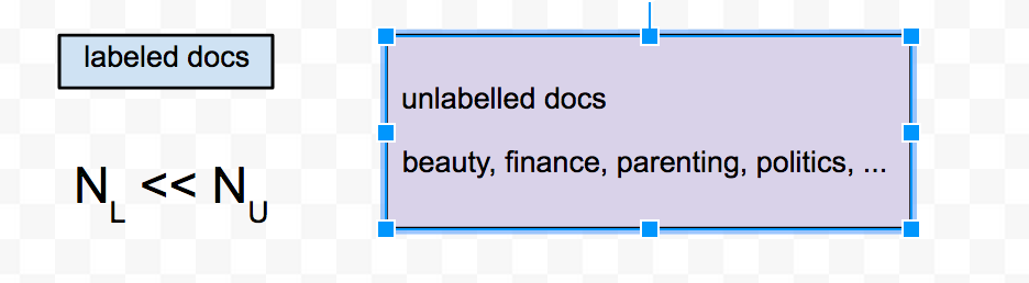
If we have a collection of consumer blogs (about finance, beauty, sports, politics, …), with some labelled documents, and large amount of unlabeled ones. We can create (1-vs-1) binary TSVM classifiers, such as finance vs beauty if we have a good way to select the unlabeled data, as described in our previous blog:
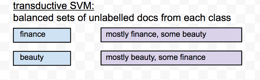
Essentially, the unlabeled documents must consist only of finance and beauty blogs, and in the same ratio as the training data.
TSVMs only work well for simple binary ( 1 vs 1 ) classification, and only when the document classes form simple clusters. They don’t work for multi-class classifier because they can not handle ( 1 vs all ) data sets.
So while TSVMs do work, not just any unlabeled data set will do. Indeed, I personally believe the key to a good TSVM is creating a well balanced unlabeled data. Or, equivalently, estimating the fraction 
UniverSVM (USVM)
In 1998, and , later in 2006, Vapnik introduced a different kind of SVM–which also the allows learning from unlabeled data–but replaces the Principle of Maximum Margin with a more robust method called
the UniverSVM: the Principle of Maximum Contradictions
The idea is to add in data from classes that are significantly different from the 2 classes being separated:
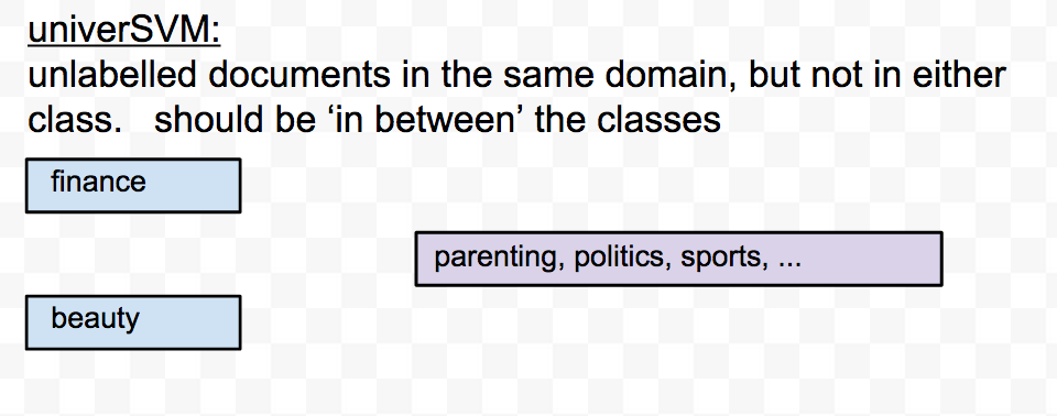
To create a finance vs beauty classifier, we would add labelled and/or unlabeled documents from other categories, such as parenting, politics, sports, etc. We then want a binary classifier that not only separates the 2 labeled classes, but is also as different from the other class–the Universum.
We create 2 replicas of the Universum–one with all (+) labels, and one all (-). We then add unlabeled documents (blue circles) that lie in the margin between classes–or really in the space between the (+/-) classes:

The best Universum examples will lie in the convex hull between the finance and beauty documents; those inside the convex hulls will most likely be ignored. Since all the u-labels are wrong, every equivalence class of hyperplanes will produce numerous contradictions on the Universum points (u):
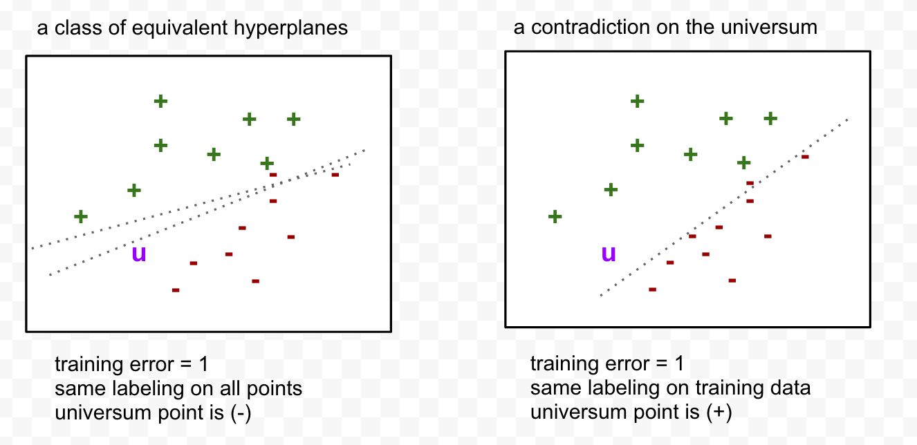
The best model has the largest diversity on the Universum; in other words, the largest VC Entropy. Vapnik has pointed out the following interpretation of the Universum: “[When trying to classify the labeled data, try to avoid extra generalizations.]”
The best model has the Maximum # of Contradictions on the Universum.
The UniverSVM (USVM) represents a kind of prior information that we add to the problem; the difference is that instead of specifying a prior distribution, which is hard, we replace this with a more practical approach–to specify a set of specific examples.
Notice we could have just created a 3-class SVM (and theUniverSVM code provides this for direct comparison). Or we could build 2-class classifier, augmented with some clustering metric to avoid the other class--in the same spirit the S4VM method. See, for example, the recent paper on EMBLEM. But in these simple approaches, the other class must only contain other–and that’s hard.
USVMs compared to TSVMs:
In the TSVM we have to be sure we are adding documents that are in the same classes as the training data. In the USVM, we must be sure we are adding documents that do not belong to either class.
Also, with a TSVM, we need to know the fraction of (+/-) documents, whereas with the USVM we don’t. The USVM would seem to admit some data from all classes–in principle. In practice, we will do much better if it does not.
Most importantly, unlike the TSVM, the USVM optimization is convex. So adding in bad data may will not cause convergence problems as in the TSVM and thus degrade the model. At least we hope.
Also, as with the TSVM, we suspect the USVM will only work for small
The UniverSVM Algorithm
The SVM approach, inspired by SLT, implements a data dependent, but distribution independent, regularizer that lets us select the best model 
the Principe of Maximum Power
A model 

Suppose we know a prior distribution 

We rarely can define 
Let us sample 

We call the practical method the UniverSVM. The key insight of the UniverSVM is that while we can not compute this integral, we can estimate it by measuring the number of contradictions the class of hyperplanes generates on points in
The Principle of Maximum Contradictions:
We need a way to select the equivalence class 
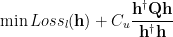
We augment the standard SVM optimization problem with a Universum regularizer

where H is the standard SVM Hinge Loss.
The regularizer 
Laplacian SVMs and the The Maximum Volume Principle
About the same time Vapnik introduced the UniverSVM, Nyogi (at the University of Chicago) introduced both the TSVM SvmLin code, as well as a new approach to Semi-Supervised learning, the Laplacian SVM (or LapSVM).
The TSVM maximizes the margin for the labelled and unlabeled data. The USVM maximizes the contradictions on the unlabeled (UniverSVM) set. In fact, both approximate a more general form of capacity–the maximum volume between the convex hulls of the data sets. And this can be approximation using Laplacian regularization! Let’s see how this all ties together.
The LapSVM optimization is

We see it is very similar to the USVM, but with a different regularizer –norm of the Graph Laplacian 
The LapSVM has recently been applied to text classification, although we dont have a C or python version of the code to test like with do with SvmLin and the UniverSVM.
LapSVMs and related Manifold Learning approaches have motivated some very recent advances in Semi-Supervised Deep Learning methods, such as the Manifold Tangent Classifier. This classifier learns the underlying manifold using contractive auto-encoder, rather than using a simple Laplacian–and this seems to work very well for images.
(We note that the popular SciKit Learn package includes Manifold Learning, but these are only the Unsupervised variants.)
We can relate the LapSVM approach to the VC-SLT, through the Principle of Maximum Volume:
the Norm of the Graph Laplacian is measure of the VC Entropy
Let us again assume we have to select the best equivalence class 


We then simply need to approximate the volume

We need a way to compute V, so we assume there exists an operator 
To this end, Vapnik et. al. introduce “a family of transductive algorithms which implement the maximum volume principle“, called Approximate Volume Regularization (AVR) algorithms(s). They take the form
For many problems,

the specific form specified by the specific AVR.
If we write the general form of

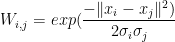
W can be defined using the Gaussian Similarity

which has a single adjustable width parameter 
A more robust Laplacian uses the Local-Scaling Similarity
which has N adjustable parameters 
the Maximum Volume Principle may be a better measure of VC capacity
This Principle of Maximum Volume has been applied in a number of ways, such as in recent papers on Maximum Volume Clustering and , and this one for Outlier Detection.
Most importantly, a very recent paper proposes a MultiClass Approximate volume Regularization Algorithm (MAVR).
We have also connected to seemingly different approaches to machine learning–traditional VC theory and operator theoretic manifold learning. In a future post, we will look at some practical examples and compares how well the available open source TSVM and USVM codes on text data.
Further Reading
Practical Conditions for Effectiveness of the Universum Learning
Practical Analysis of the Universum SVM Learning
Advances in Universum Learning
Thesis: Analysis and extensions of Universum learning (2014)

This comment is based on a few posts you had on RBS. I am confused.
Just to give an example of one stumbling block (for me), you tried to show that the function being minimized for an RBM had both an entropy and an energy component. I did not understand what ‘entropy’ meant in this context. Does it mean “disorder” is minimized? “information” is maximized? And if so, what disorder, or what information? With energy as well, did it mean that incompatibilities (such as incompatible spins in a spin glass) are minimized? If so, what incompatibilities?
And I didn’t quite understand why having vast number of hidden units makes for a more convex energy landscape. Does it have something to do with ‘degrees of freedom’ or with more ways existing of reaching a solution?
Could you suggest some topics that I should read before reading your blog – so that your blog makes more sense to me. It looks fascinating.
LikeLike