Don’t Peek part 2: Predictions without Test Data

This is a followup to a previous post:

DON’T PEEK: DEEP LEARNING WITHOUT LOOKING … AT TEST DATA

The idea…suppose we want to compare 2 or more  deep neural networks (DNNs). Maybe we are

• fine tuning a DNN for transfer learning, or
• comparing a new architecture to an old on, or
• we are just tuning our hyper-parameters.

Can we determine which DNN will generalize best–without peeking at the test data?

Theory actually suggests–yes we can!

An Unsupervised Test Metric for DNNs

We just need to measure the average log norm of the layer weight matrices 

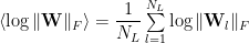
where  is the Frobenius norm

The Frobenius norm is just the sum of the square of the matrix elements. For example, it is easily computed in numpy as

np.linalg.norm(W,ord='fro')

where ‘fro’ is the default norm.

It turns out that  is amazingly correlated with the test accuracy of a DNN.  How do we know ?  We can plot   vs the reported test accuracy for the  pretrained DNNs, available in PyTorch.   First, we look at the VGG models:

VGG and VGG_BN models

The plot shows the 4 VGG and VGG_BN models. Notice we do not need the ImageNet data to compute this; we simply compute the average log Norm and plot with the (reported Top 5) Test Accuracy.  For example, the orange dots show results for the pre-trained VGG13 and VGG13_BN ImageNet models.  For each pair of models, the larger the  Test Accuracy, the smaller  .    Moreover, the correlation is nearly linear across the entire class of VGG models.  We see similar behavior for …

the ResNet models

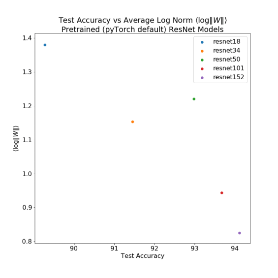
Across 4/5 pretrained ResNet models, with very different sizes, a smaller   generally implies a better Test Accuracy.

It is not perfect–ResNet 50 is an outlier–but it works amazingly well across numerous pretrained models, both in pyTorch and elsewhere (such as the OSMR sandbox).  See the Appendix for more plots.  What is more, notice that

the log Norm metric  is completely Unsupervised

Recall that we have not peeked at the test data–or the labels.  We simply computed for the pretrained models directly from their weight files, and then compared this to the reported test accuracy.

Imagine being able to fine tune a neural network without needing test data.  Many times we barely have enough training data for fine tuning, and there is a huge risk of over-training. Every time you peek at the test data, you risk leaking information into the model, causing it to overtrain. It is my hope this simple but powerful idea will help avoid this and advance the field forward.

Why does this work ? 

Applying VC Theory of Product Norms

A recent paper by Google X and MIT shows that there is A Surprising Linear Relationship [that] Predicts Test Performance in Deep Networks.  The idea is to compute a VC-like data dependent complexity metric — — based on the Product Norm of the weight matrices:

Usually we just take  as the Frobenius norm (but any p-norm may do)

If we take the log of both sides, we get the sum

So here we just form the average log Frobenius Norm as measure of DNN complexity, as suggested by current ML theory

And it seems to work remarkably well in practice.

Log Norms and Power Laws

We can also understand this through our Theory of Heavy Tailed Implicit Self-Regularization in Deep Neural Networks.

The theory shows that each layer weight matrix of (a well trained) DNNs resembles a random heavy tailed matrix, and we can associate with it a power law exponent

The exponent characterizes how well the layer weight matrix represents the correlations in the training data.  Smaller is better.

Smaller exponents correspond to more implicit regularization, and, presumably, better generalization (if the DNN is not overtrained).  This suggests that the average power law would make a good overall unsupervised complexity metric for a DNN–and this is exactly what the last blog post showed.

The average power law metric is a weighted average,

where the layer weight factor should depend on the scale of . In other words, ‘larger’ weight matrices (in some sense) should contribute more to the weighted average.

Smaller  usually implies better generalization

For heavy trailed matrices, we can work out a relation between the log Norm of and the power law exponent :

where we note that

So the weight factor is simply the log of the maximum eigenvalue associated with 

In the paper will show the math; below we present numerical results to convince the reader.

This also explains why Spectral Norm Regularization Improv[e]s the Generalizability of Deep Learning.  The smaller  gives a smaller power law contribution, and, also, a smaller log Norm.  We can now relate these 2 complexity metrics:

We argue here that we can approximate the average Power Law metric  by simply computing the average log Norm of the DNN layer weight matrices.   And using this,  we can actually predict the trends in generalization accuracy — without needing a test data set!

Discussion and Conclusion

Implications: Norms vs Power Laws

The Power Law metric is consistent with the recent theoretical results, but our approach and the intent is different:

• Unlike their result, our approach does not require modifying the loss function.
• Moreover, they seek a Worst Case complexity bound.  We seek Average  Case metrics.  Incredibly, the 2 approaches are completely compatible.

But the biggest difference is that we apply our Unsupervised metric to large, production quality DNNs.

We believe this result will have large applications in hyper-parameter fine tuning DNNs.  Because we do not need to peek at the test data, it may prevent information from leaking from the test set into the model, thereby helping to prevent overtraining and making fined tuned DNNs more robust.

WeightWatcher

We have built a python package for Jupyter Notebooks that does this for you–the weight watcher.  It works on Keras and PyTorch.  We will release it shortly.

Please stay tuned!  And please subscribe if this is useful to you.

---

Appendix:

• A1.  More Results
• A2.  Numerical Test of Log Norm Power Law Relations
• A3.  Proof of the Log Norm Power Law Relation (N/A…will redo soon)

---

A1.  More Results

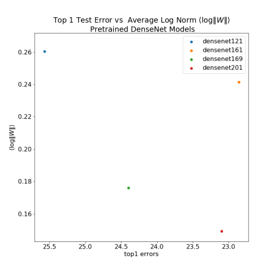
We use the OSMR Sandbox to compute the average log Norm for a wide variety of DNN models, using pyTorch, and compare to the reported Top 1 Errors.  This notebook reproduces the results.

All the ResNet Models

DenseNet

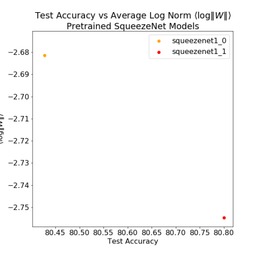
SqueezeNet

DPN

SeResNet

---

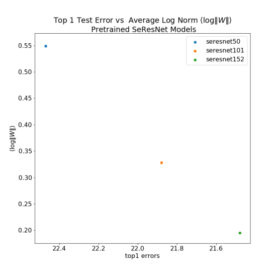
A2.  Numerical Test of Log Norm Power Law Relations

In the plot below, we generate a number of heavy tailed matrices, and fit their ESD to a power law.  Then we compare

The code for this is:

N, M, mu = 100, 100, 2.0

W = np.random.pareto(a=mu,size=(N,M))

normW = np.linalg.norm(W)

logNorm2 = 2.0*np.log10(normW)

X=np.dot(W.T,W)/N

evals = np.linalg.eigvals(X)

l_max, l_min = np.max(evals), np.min(evals)

fit = powerlaw.Fit(evals)

alpha = fit.alpha

ratio = logNorm2/np.log10(l_max)

Below are results for a variety of heavy tailed random matrices:

The plot shows the relation between the ratios and the empirical power law exponents . There are three striking features; the linear relation

• is very clear for
• saturates for  for large M
• extends beyond  because of finite size effects

A3.  Proof of the Power Law –  Log Norm  Relations

In our next paper, we will drill into these details and explain further how this relation arises and the implications for Why Deep Learning Works.

---