Another Holiday Blog: Feedback and Questions are very welcome.
I have a client who is using Naive Bayes pretty successfully, and the subject has come up as to ‘why do we need fancy machine learning methods?’ A typical question I am asked is:
Why do we need Regularization ?
What happens if we just turn the regularizer off ?
Can we just set it to a very small, default value ?
After all, we can just measure what customers are doing exactly. Why not just reshow the most popular items, ads, etc to them. Can we just run a Regression? Or Naive Bayes ? Or just use the raw empirical estimates?
Do we Need Hundreds of Classifiers to Solve Real World Classification Problems?
Sure, if you are simply estimating historical frequencies, n-gram statistics, etc, then a simple method like Naive Bayes is fine. But to predict the future..
the Reason we need Regularization is for Generalization.
After all, we don’t just want to make the same recommendations over and over.
 Unless you are just in love with ad re-targeting (sic). We want to predict on things we have never seen.
And we need to correct for presentation bias when collecting data on things we have seen.
Most importantly, we need methods that don’t break down unexpectedly.
In this post, we will see why Regularization is subtle and non-trivial even in seemingly simple linear models like the classic Tikhonov Regularization. And something that is almost never discussed in modern classes.
We demonstrate that ‘strong’ overtraining is accompanied by a Phase Transition–and optimal solutions lies just below this.
The example is actually motivated by something I saw recently in my consulting practice–and it was not obvious at first.

Still, please realize–we are about to discuss a pathological case hidden in the dark corners of Tikhonov Regularization–a curiosity for mathematicians.
See this Quora post on SVD in NLP for some additional motivations.
Let’s begin when Vapnik [1], Smale [2], and the other great minds of the field begin:
(Regularized) Linear Regression:
The most basic method in all statistics is linear regression


It is attributed to Gauss, one of the greatest mathematicians ever.
One solution is to assume Gaussian noise and minimize the error.
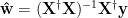
The solution can also be constructed using the Moore-Penrose PseudoInverse.
If we multiply by 

The formal solution is
which is only valid when we can actually invert the data covariance matrix 
We say the problem is well-posed when

- exists,
- is unique, and
- is stable.
Otherwise we say it is singular, or ill-posed [1].
In nearly all practical methods, we would not compute the inverse directly, but use some iterative technique to solve for 
Frequently XTX can not be inverted..or should not be inverted..directly.
Tikhonov Regularization
A trivial solution is to simply ‘regularize’ the matrix

Naively, this seems like it would dampen instabilities and allow for a robust numerical solution. And it does…in most cases.
If you want to sound like you are doing some fancy math, give it a Russian name; we call this Tikhonov Regularization [4]:

 This is (also) called Ridge Regression in many common packages such as scikit learn.
The parameter 
Grid searching
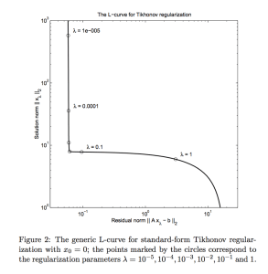
The L-curve is a log-log plot of the the norm of the regularized solution vs. the norm of the residual. The best
This challenge of regularization is absent from basic machine learning classes?
The optimal 
We might naively imagine
The regularization fails in these 2 notable cases, when
- the model errors are correlated, which fools simple cross validation
-
and the number of features ~ the number of training instances, which leads to a phase transition.
Today we will examine this curious, spurious behavior in case 2 (and look briefly at 1)
Regimes of Applications

As von Neumann said once, “With four parameters I can fit an elephant, and with five I can make him wiggle his trunk”
To understand where the regularization can fail, we need to distinguish between the cases in which Ridge Regression is commonly used.
Say we have 


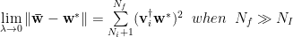
High Variance: 
This regime is overdetermined, complicated models that are subject to overtraining. We find multiple solutions which satisfy our constraints.
Most big data machine learning problems lie here. We might have 100M documents and 100K words. Or 1M images and simply all pixels as the (base) features.

Regularization lets us pick the best of solution which is the most smooth (L2 norm), or the most sparse (L1 norm), or maybe even the one with the least presentation bias (i.e. using Variance regularization to implement Counterfactural Risk Minimization)
High Bias regime: 
This is the Underdetermined regime, and any solution we find, regularized or not, will most likely generalize poorly.
When we have more instances than features, there is no solution at all (let alone a unique one)

Still, we can pick a regularizer, and the effect is similar to dimensional reduction. Tikhonov Regularization is similar truncated SVD (explained below)
Any solution we find may work, but the predictions will be strongly biased towards the training data.
But it is not only just sampling variability that can lead to poor predictions.
In between these 2 limits is an seemingly harmless case, however, this is really a
Danger Zone: 
 This is a rare case where the number of features = the number of instances.
This does come up in practical problems, such as classifying a large number of small text phrases. (Something I have been working on with one of my larger clients)

The number of phrases ~ the number of unique words.
This is a dangerous case … not only because it seems so simple … but because the general theory breaks down. Fortunately, it is only pathologicial in
The limit of zero regularization
We examine how these different regimes behave for small values of
Let’s formalize and consider the how the predicted accuracy behaves.
The Setup: An Analytical Formulation
We analyze our regression under Gaussian noise 

where


This simple model lets us analyze predicted Accuracy analytically.
Let


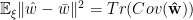
![\mathbf{\bar{w}}=\mathbb{E}_{\xi}[\mathbf{\hat{w}}]](https://s0.wp.com/latex.php?latex=%5Cmathbf%7B%5Cbar%7Bw%7D%7D%3D%5Cmathbb%7BE%7D_%7B%5Cxi%7D%5B%5Cmathbf%7B%5Chat%7Bw%7D%7D%5D+&bg=%23ffffff&fg=%23000000&s=0&c=20201002)
We would like define, and the decompose, the Generalization Accuracy into Bias and Variance contributions.
Second, to derive the Generalization Error, we need to work out how the estimator behaves as a random variable. Frequently, in Machine Learning research, one examines the worst case scenario. Alternatively, we use the average case.
Define the Estimation Error

Notice that by Generalization Error, we usually we want to know how our model performs on a hold set or test point 
![\mathbb{E}_{\mathbf{\xi}}[(\mathbf{x^{\dagger}}(\hat{\mathbf{w}}-\mathbf{w^{*}}))^{2}]](https://s0.wp.com/latex.php?latex=%5Cmathbb%7BE%7D_%7B%5Cmathbf%7B%5Cxi%7D%7D%5B%28%5Cmathbf%7Bx%5E%7B%5Cdagger%7D%7D%28%5Chat%7B%5Cmathbf%7Bw%7D%7D-%5Cmathbf%7Bw%5E%7B%2A%7D%7D%29%29%5E%7B2%7D%5D+&bg=%23ffffff&fg=%23000000&s=0&c=20201002)
In the Appendix, we work out the generalization bounds for the worst case and the average case. From here on, however, when we refer to Generalization Error, we mean the average case Estimation Error (above).
Bias-Variance Tradeoff
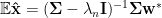
For Ridge Regression, the mean estimator is

and its variation is

We can now decompose the Estimation Error into 2 terms:


and examine each regime in the limit
The Bias is just the error of the average estimator:

and the Variance is the trace of the Covariance of the estimator

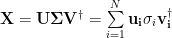
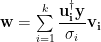
We can examine the limiting behavior of these statistics by looking at the leading terms in a series expansion for each. Consider the Singular Value Decomposition (SVD) of


Let 

We can write the Bias as

With no regularization, and the number of features exceeds the number of instances, there is a strong bias, determined by the ‘extra’ singular values
Otherwise, the Bias vanishes.
So the Bias appears to only matter in the underdetermined case.
(Actually, this is misleading; in the overdetermined case, we can introduce a bias when tuning the regularization parameter too high)
In contrast, the Variance


can diverge if the minimal singular value is small:

That is, if the singular values decrease too fast, the variance can explode.
And this can happen in the danger zone
When 
Which also means the Central Limit Theorem (CLT) breaks down…at least how we normally use it.
Traditionally, the (classical) CLT says that the infinite sum of i.i.d. random variables 


These power-law distributions are quite interesting–and arise frequently in chemistry and physics during a phase transition. But first, let’s see the divergent behavior actually arise.
When More is Less: Singularities
Ryota Tomioka [3] has worked some excellent examples using standard data sets

[I will work up some ipython notebook examples soon]
The Spambase dataset is a great example. It has 

![N_{i}\in(0,4601]](https://s0.wp.com/latex.php?latex=N_%7Bi%7D%5Cin%280%2C4601%5D+&bg=%23ffffff&fg=%23000000&s=0&c=20201002)

As the data set size 
Many other datasets show this anomalous behavior at 
Ridge Regression vs Logistic Regression: Getting out of the Hole
Where Ridge Regression fails, Logistic Regression bounces back. Below we show some examples of RR vs LR in the
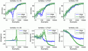
Logistic Regression still has problems, but it no where near as pathological as RR.
The reason for this is subtle.
- In Regression, the variance goes to infinity
- In Classification, the norm
goes to infinity
Traditional ML Theory: Isn’t the Variance Bounded?
Traditional theory (very losely) bounds for quantities like the generalization error and (therefore) the variance.
We work out some of examples in the Appendix.
Clearly these bounds don’t work in all cases. So what do they really tell us? What’s the point?
These theories gives us some confidence that we can actually apply a learning algorithm–but only when the regularizer is not too small and the noise is not too large.
They essentially try to get us far away from the pathological phase transition that arises when the variance diverges.
Cross Validation and Correlated Errors

In practice, we would never just cross our fingers set 
We pick a hold out set and run Generalized Cross Validation (GCV) . Yet this can fail when
- the model errors
are not i.i.d. but are strongly correlated
- we don’t know what accuracy metric to use?
Hansen [5, 7] has discussed these issue in detail…and he provides an alternative method, the L-curve, which attempt to balance the size of the regularized solution and the residuals.

For example, we can sketch the relative errors 
In other words, while most packages provide a small choice of regression metrics; as data scientists, the defaults like
Hansen claims that,”experiments confirm that whenever GCV finds a good regularization parameter, the corresponding solution is located at the corner of the L-curve.” [7]
This means that the optimal regularized solution lives ‘just below’ the phase transition, where the norm diverges.
Phase Transitions in Regularized Regression

What do we mean by a phase transition?
The simplest thing is to we plot a graph and look a steep cliff or sharp change.
Here, generalization accuracies drops off suddenly as

In a physical phase transition,the fluctuations (i.e. variances and norms) in the system approach infinity.
Imagine watching a pot boil

We see bubbles of all sizes, small and large. The variation in bubble size is all over the map. This is characteristic of a phase transition: i.e. water to gas.
When we cook, however, we frequently simmer our foods–we keep the water just below the boiling point. This is as hot as the water can get before it changes to gas.
Likewise, it appears that in Ridge Regression, we frequently operate at a point just below the phase transition–where the solution norm explodes. And this is quite interesting. And, I suspect, may be important generally.
In chemical physics, we need special techniques to treat this regime, such as the Renormalization Group. Amazingly, Deep Learning / Restricted Boltzmann Machines look very similar to the Variational Renormalization Group method.
In our next post, we will examine this idea further, by looking at the phase diagram of the traditional Hopfield Neural Networ, and the idea of Replica Symmetry Breaking in the Statistical Mechanics of Generalization. Stay tuned !
References
1. Vapnik and Izmailov, V -Matrix Method of Solving Statistical Inference Problems, JMLR 2015
2. Smale, On the Mathematical Foundations of Learning, 2002
3. Tomioka, Class Lectures on Ridge Regression,
4. http://ttic.uchicago.edu/~gregory/courses/LargeScaleLearning/lectures/proj_learn1.pdf
5. The L-curve and its use in the numerical treatment of inverse problems
6. Discrete Ill-Posed and Rank Deficient Problems
7. The use of the L-curve in the regularization of discrete ill-posed problems, 1993
Appendix: some math
Bias-Variance Decomposition

when ![\mathbb{E}[\mathbf{\xi}]=0](https://s0.wp.com/latex.php?latex=%5Cmathbb%7BE%7D%5B%5Cmathbf%7B%5Cxi%7D%5D%3D0+&bg=%23ffffff&fg=%23000000&s=0&c=20201002)
then

Let

be the data covariance matrix. And , for convenience, let

The Expected value of the optimal estimator, assuming Gaussian noise, is given using the Penrose Pseudo-Inverse
The Covariance is

The regularized Covariance matrix arises so frequently that we will assign it a symbol

We can now write down the mean and covariance
[more work needed here]
Average and Worst Case Generalization Bounds
Consider the Generalization Error for a test point
![\mathbb{E}_{\mathbf{\xi}}[(\mathbf{x^{\dagger}}(\hat{\mathbf{w}}-\mathbf{w^{*}}))^{2}] =\lambda^{2}_{n}[\mathbf{x^{\dagger}}\mathbf{\Sigma}_{\lambda_{n}}^{-1}\mathbf{w}]^{2}+\dfrac{\sigma^{2}_{n}}{n}\mathbf{x^{\dagger}}\mathbf{\Sigma}_{\lambda_{n}}^{-1}\mathbf{\Sigma}\mathbf{\Sigma}_{\lambda_{n}}^{-1}\mathbf{w}](https://s0.wp.com/latex.php?latex=%5Cmathbb%7BE%7D_%7B%5Cmathbf%7B%5Cxi%7D%7D%5B%28%5Cmathbf%7Bx%5E%7B%5Cdagger%7D%7D%28%5Chat%7B%5Cmathbf%7Bw%7D%7D-%5Cmathbf%7Bw%5E%7B%2A%7D%7D%29%29%5E%7B2%7D%5D+%3D%5Clambda%5E%7B2%7D_%7Bn%7D%5B%5Cmathbf%7Bx%5E%7B%5Cdagger%7D%7D%5Cmathbf%7B%5CSigma%7D_%7B%5Clambda_%7Bn%7D%7D%5E%7B-1%7D%5Cmathbf%7Bw%7D%5D%5E%7B2%7D%2B%5Cdfrac%7B%5Csigma%5E%7B2%7D_%7Bn%7D%7D%7Bn%7D%5Cmathbf%7Bx%5E%7B%5Cdagger%7D%7D%5Cmathbf%7B%5CSigma%7D_%7B%5Clambda_%7Bn%7D%7D%5E%7B-1%7D%5Cmathbf%7B%5CSigma%7D%5Cmathbf%7B%5CSigma%7D_%7B%5Clambda_%7Bn%7D%7D%5E%7B-1%7D%5Cmathbf%7Bw%7D+&bg=%23ffffff&fg=%23000000&s=0&c=20201002)
We can now obtain some very simple bounds on the Generalization Accuracy (just like a bona-a-fide ML researcher)
The worst case bounds
![[\mathbf{x^{\dagger}}\mathbf{\Sigma}_{\lambda_{n}}^{-1}\mathbf{w}]^{2}\le\Vert\mathbf{\Sigma}_{\lambda_{n}}^{-1}\mathbf{x}\Vert^{2}\Vert\mathbf{w^{*}}\Vert^{2}](https://s0.wp.com/latex.php?latex=%5B%5Cmathbf%7Bx%5E%7B%5Cdagger%7D%7D%5Cmathbf%7B%5CSigma%7D_%7B%5Clambda_%7Bn%7D%7D%5E%7B-1%7D%5Cmathbf%7Bw%7D%5D%5E%7B2%7D%5Cle%5CVert%5Cmathbf%7B%5CSigma%7D_%7B%5Clambda_%7Bn%7D%7D%5E%7B-1%7D%5Cmathbf%7Bx%7D%5CVert%5E%7B2%7D%5CVert%5Cmathbf%7Bw%5E%7B%2A%7D%7D%5CVert%5E%7B2%7D+&bg=%23ffffff&fg=%23000000&s=0&c=20201002)
The average case bounds
![\mathbb{E}_{\mathbf{w^{*}}}[\mathbf{x^{\dagger}}\mathbf{\Sigma}_{\lambda_{n}}^{-1}\mathbf{w}]^{2}\le\alpha^{-1}\Vert\mathbf{\Sigma}_{\lambda_{n}}^{-1}\mathbf{x}\Vert^{2}](https://s0.wp.com/latex.php?latex=%5Cmathbb%7BE%7D_%7B%5Cmathbf%7Bw%5E%7B%2A%7D%7D%7D%5B%5Cmathbf%7Bx%5E%7B%5Cdagger%7D%7D%5Cmathbf%7B%5CSigma%7D_%7B%5Clambda_%7Bn%7D%7D%5E%7B-1%7D%5Cmathbf%7Bw%7D%5D%5E%7B2%7D%5Cle%5Calpha%5E%7B-1%7D%5CVert%5Cmathbf%7B%5CSigma%7D_%7B%5Clambda_%7Bn%7D%7D%5E%7B-1%7D%5Cmathbf%7Bx%7D%5CVert%5E%7B2%7D+&bg=%23ffffff&fg=%23000000&s=0&c=20201002)
where we assume the ‘covariance*’ is
![\mathbb{E}_{\mathbf{w^{*}}}[\mathbf{w^{*}w^{*\dagger}}]=\alpha^{-1}\mathbf{I}](https://s0.wp.com/latex.php?latex=%5Cmathbb%7BE%7D_%7B%5Cmathbf%7Bw%5E%7B%2A%7D%7D%7D%5B%5Cmathbf%7Bw%5E%7B%2A%7Dw%5E%7B%2A%5Cdagger%7D%7D%5D%3D%5Calpha%5E%7B-1%7D%5Cmathbf%7BI%7D+&bg=%23ffffff&fg=%23000000&s=0&c=20201002)
Discrete Picard Condition
We can use the SVD approach to make stronger statements about our ability to solve the inversion problem

I will sketch an idea called the “Discrete Picard Condition” and provide some intuition
Write 
Introduce an abstract PseudoInverse, defined by

Express the formal solution as

Imagine the SVD of the PseudoInverse is

and use it to obtain

For this expression to be meaningful, the SVD coefficients 

Consequently, the only coefficients that carry any information are larger than the noise level. The small coefficients have small singular values and are dominated by noise. As the problem becomes more difficult to solve uniquely, the singular values decay more rapidly.
If we discard the 
Truncated SVD
which is similar in spirit to spectral clustering.

Nice post! Another good take on the underdetermined regime, with a Bayesian angle to it:
https://jakevdp.github.io/blog/2015/07/06/model-complexity-myth/
LikeLike
Excellent blog. I wish everyone explained technical concepts so well
LikeLike
Thanks
LikeLike
wow, this post is amazing! Though I wish in practice we could just cross our fingers and set \lambda=0.00000001. Parameter tuning is so frustrating!
LikeLike
Very thoughtful presentation. May I offer a simple insight from a Physics perspective, and with many years of work in diverse sensor and imaging problems. If solving the problem requires regularization, then your model is wrong. Serious problems often resist solution; and resistance to solution is often very stubborn. Experience shows trying Singular Value Decomposition often helps diagnose what is wrong with a problem, or a model, or particular data. Sometimes SVD works so well, I abandon regularization altogether.
LikeLike
Thanks. This interesting case actually came up in a production system with a client when trying to apply Ridge Regression. Usually I would just use Logistic Regression or and SVM. What I have found in text classification is that the SVM regularization parameter is universal. Which is not really discussed in the ML literature.
LikeLike
I agree…regularization seems like a hack.
LikeLike
Is there a typo in definitions of high variance and high bias regimes?
For high variance you are writing Nf >> NI, and for high bias Nf << NI.
I think it should be the other way around.
LikeLike
OK, my mistake. I think the definitions of high bias and high variance are OK. But what confuses me is your use of overdetermined and underdetermined terms. For example for high bias case (Nf<<NI), you say that this is underdetermined regime. But then you say that ‘When we have more features than instances, there is no solution at all’. I think the high bias case is overdetermined. If in Xw=y, each row is an instance and columns are for features, we have more equations than unknowns, so it should be overdetermined.
LikeLike
there might be typo…thanks I’ll review
LikeLike