Foundations: Theory of Compressed Sensing

Introduction:

In an much earlier post, we looked at detecting Gravity Waves using Machine Learning and  techniques like Minimum Path Basis Pursuit.  

SciKit Learn even has a version of this called Orthogonal Matching Pursuit

Here, we drill down into the theoretical justifications of the general approach–called Compressed Sensing–ala Terrance Tao.

Linear Algebra: Solving Ax=b with an Over-Complete Basis

In traditional linear algebra, we solve the problem

using the Penrose Pseudo-Inverse

where is a vector of length , and is an m x n matrix

A standard and very old machine learning approach is to add a small constant to the diagonal, called  Tikhonov Regularization or Ridge Regression

This is equivalent to constrained optimization problem.

Ridge Regression in available in SciKit Learn

Basis Pursuit — or L1 Regularization

It has been known in geophysics and astrophysics since the 1970s that frequently we can do better if we minimize the -norm instead of the  -norm of

where

Note: sometimes this is written as an unconstrained optimization problem

subject to 

appland this can be relaxed to

subject to 

The constrained solution, and related -regularization problems, are readily solved using numerical techniques, and are available, in some form, in many R and MatLab packages and open source tools.

Other Open Source Tools

Technically, Compressed sensing means we sample the basis set / features randomly, and then apply L1 regularization.  This is very useful for problems like image reconstruction.

But we can also just apply L1 regularization directly to discrete features.  Lasso Regression.  L1-regularized SVMs. They are not exactly the same, but practically it is quite useful.  I remember a time when having access to an L1-regularized method was a big deal. So I am going to be a little loose here, and tighten up the theory in the next post (on statistical mechanics of compressed sensing)

Liblinear: (L1 Regularized Classification)

The current version of Liblinear (1.9) includes -regularization for classification in (along with -regularization SVM regression methods ):

./liblinear-1.91/train 
Usage: train [options] training_set_file [model_file]
options:
-s type : set type of solver (default 1)
...
5 -- L1-regularized L2-loss support vector classification
...

To solve a regression, we can use

Vowpal Wabbit (VW):

VW actually solves the more general problem (i.e. an Elastic Net)

where is a general Loss function for either classification or regression.  We set the regularization parameters via the command line Update Rule Options

--l1 arg (=1)                    l_1 lambda
--l2 arg (=1)                    l_2 lambda

There even hardware implementations of compressed sensing: see the awesome Nuit Blanche blog for more details.

(Apparently) when solving a regression problem, we call the -regularization problem Basis Pursuit (BP) [7]

BP is a principle for decomposing a signal into an optimal superposition of dictionary elements (an over-complete basis), where optimal means having the smallest -norm of coefficients among all such decompositions.

Unfortunately, neither of these off-the-shelf programs will work to find our Gravity Waves; for that, we need to add path constraints.  

Our signal is very weak (SNR << 1) and we are trying to reconstruct a continuous, differentiable function of a known form.  We  will be push the computational and theoretical limits of these methods.  To get there (and because it is fun), we highlight a little theoretical work on Compressed Sensing

Compressed Sensing

In the past decade, work by Dave Donoho and Emmanuel Candes at Stanford and Terence Tao at Berkeley have formalized and developed the theoretical and practical ideas of Basis Pursuit under the general name compressed sensing.

A common use of compressed sensing is for image reconstruction

Beyond the Sampling Theorem

To reconstruct a signal , we used to think we were bandwidth limited; this is the essence of the Nyquist–Shannon Sampling Theorem

Tao, a former child prodigy who won the Fields Medal in 2006, took some time off from pure math to show us that we are, in fact, limited by the signal structure, not the bandwidth.

We call  S-sparse when at most only S of the coefficients can be non-zero (.   For example, many images are S-sparse in a wavelet basis; this is the basis of the newer JPEG2000 algorithm.

This allows us to reconstruct a signal with as few data as possible–if we can guess the right basis.

Ideal Sparse Reconstruction

In an ideal world, we would like to find the most sparse solution, which means we solve the regularization problem

 subject to 

where the norm is just the number of non-zero components.

This is very difficult to achieve numerically.  It turns out that we can approximate this problem with the  regularization problem, which can be solved as a convex optimization problem.   And we even have some ideas why. But why ask why?

IMHO, applied machine learning work requires applying off-the-shelf tools, even in seemingly impossible situations, and yet avoiding wasting effort on hopeless methods.  The best applied scientists understand the limits of both the methods they use and the current underlying theory.

Theoretical Justifications for Compressed Sensing

Any early idea showed that we can, in fact, do better than the Sampling Theorem just using random projections:

Theorem (Candes-Romber  2004):

Suppose we choose m points randomly out of n.  Then, with high probability, every S-sparse signal  can be reconstructed from , so long as for some absolute constant C.

This result leads hope that this can be formalized.  But what kind of conditions do we need on to at least have a hope of reconstructing ?  A very simple result is

Proposition:

Suppose that any columns of matrix are linearly independent. (This is a reasonable assumption once .) Then, any S-sparse signal can be reconstructed uniquely from .

Proof:

Suppose not; then there are two S-sparse signals with .  This implies But is 2S-sparse, so there is a linear dependence between 2S columns of .  A contradiction.

So we might expect, on a good day. that every 2S columns of A are linearly independent.   In fact, we can say a little more

Conditions on A and the Restricted Isometry Property (RIP)

There are now several theoretical results ensuring that Basis Pursuit works whenever the measurement matrix is sufficiently “incoherent”, which roughly means that its matrix entries are uniform in magnitude.

In practice, numerical experiments suggest that most S-sparse signals can be recovered exactly when

This means we can strengthen the proposition above by requiring, for example, that every 4S columns of are approximately orthonormal.  It turns out that many well known Random Matrices satisfy this property, such as Gaussian Random Matrices.

Technically, the RIP is stated as:

Suppose that there exists a constant  such that, for every m × s submatrix  of  and for every vector we have

whenever

If the matrix satisfies some form of RIP, we can get a theoretical upper bound on how well the BP will perform.    A basic result shows that true (i.e. RMS) error in the reconstructed signal is bounded by the  (i.e. absolute) sample error:

Theorem (Candes-Romber-Tao):

The tightest bound is due to Foucart, who shows that this bound holds when

The astute reader will recognize that the RIP asks that the signal be sparse in an orthonormal basis and that the data matrix be uniformly incoherent.    

Is this good enough?  Have you ever seen a uniformly incoherent distribution in a real world data set?

D-RIP

Many signals may in-fact, be only sparse in the non-orthogonal, overcomplete basis.   Recently, it has been shown how to define a D-RIP property [10,11] that applies to the more general case of even when the matrix is not as incoherent as we might expect or desire.

In some earlier posts, we introduced the Regularization (or Projection) Operator as a way to get at What a Kernel is (really). Recall that to successfully apply a Kernel, the associated, infinite order expansion should converge rapidly. 

Likewise, here we define a similar Operator, , that projects our sample data into the Hilbert Space, or Signal Domain .

 It is in this space that the signal is expanded in the over-complete basis

We might also refer to as a frame, although I skipping this technical detail for now.  Essentially, this means that any  infinite order expansion in converges rapidly enough that we can use it as a basis in our infinite dimensional space.

We can now adjust the RIP, extending the notion of considering every m × s submatrix to considering , the union of all subspaces spanned by all subsets  of size s.

Technically, the D-RIP is stated as:

Suppose that there exists a constant  such that 

whenever

Similarly to the RIP, Guassian, subgaussian, and Bernoulli matrices satisfy the D-RIP with m ≈ s log(d/s). Matrices with a fast multiply (DFT with random signs) also satisfy the D-RIP with m approximately of this order.

There is also a known bound.

D-RIP Bound for Basis Pursuit (Needell, Stanford 2010):

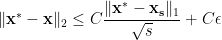
Let D be an arbitrary tight frame and let A be a measurement matrix satisfying D-RIP with δ2s < 0.08. Then the solution to -analysis satisfies

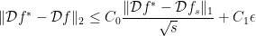
The result says that -regularization/analysis is very accurate when converges quickly (has rapidly decaying coefficients)

This is the case in applications using Wavelets, Curvelets, and Chirplets.

Warning: Don’t just use Random Features  

This does not say that we can use any random or infinite size basis.  In particular, if we combine 2 over-complete basis sets, we might overtrain or, worse, fit a spurious, misleading signal.  Been there, seen that.  This is way too common in applied work, and is also the danger we face in trying to detect a weak signal in a sea of noise.  And this is why we will add additional constraints.

Weak Signal Detection: an example

Recall that we wish to detect a very weak signal of the general form

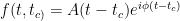
in a sea of noise,  where is a slowly varying function, and is some oscillatory function of unknown frequency, phase, and envelope.  We need to detect the presence of —and the unknown critical time .  We might be tempted to first think we can just create an overcomplete basis of functions  for variety of critical times and solve the Basis Pursuit problem.

This will most likely fail for 2 reasons

1. each critical time defines a unique -frame, and we probably should not combine all basis sets / frames in the same optimization
2. even for a single pass of BP,  there is just too much incoherent noise and/or perhaps even some other, transiently stable, detectable, but spurious signal.

Given these conditions,   one might expect a clever, adaptive or matching pursuit-like approach to work better than vanilla constrained optimization (I’ll explain the difference in a bit).  Recent research [12] indicates, however, that while we might believe

Folk Theorem:  The estimation error one can get by using a clever adaptive sensing scheme is far better than what is achievable by a nonadaptive scheme.

that, in fact,

Surprise:  The folk theorem is wrong in general. No matter how clever the adaptive sensing mechanism, no matter how intractable the estimation procedure, in general [one can not do better than] a  random projection followed by  minimization.

with the

Caveat:  “This ‘negative’ result should not conceal the fact that adaptivity may help tremendously if the SNR [Signal-to-Noise Ratio]  is sufficiently large

In a future post, we will take a second look at the theory–using Statistical Mechanics.

References

[1] 1995 Mann & Haykin, The Chirplet Transform: Physical Considerations

[2] 2004 Emmanuel Candes &  Terence Tao,  Near Optimal Signal Recovery From Random Projections: Universal Encoding Strategies?

[3] 2006  Candes, Charlton, & Helgason, Detecting Highly Oscillatory Signals by Chirplet Path PursuitThe Chirplet Transform: Physical Considerations

[4] 2008 Greenberg & Gosse, Chirplet approximation of band-limited, real signals made easy

[5] 2008, NTNU’s Onsager Lecture, Compressed Sensing by Terence Tao, part 1 of 7

[6] 2009 Tao, Compressed Sensing

[7] Chen & Donoho, Basis Pursuit

[8]  2004  Candes, Chirplets: Multiscale Recovery and Detection of Chirps

[9]  VideoLectures by Candes

[10] 2010 Emmanuel J. Candes, Yonina C. Eldar, Deanna Needell, Paige Randall,  Compressed Sensing with Coherent and Redundant Dictionaries

[10a] http://www.cmc.edu/pages/faculty/DNeedell/RhodesTalk.pdf

[11] 2012 Mark A. Davenport, Deanna Needell, Michael B. Wakin, Signal Space CoSaMP for Sparse Recovery with Redundant Dictionaries

[12] 2012 Arias-Castro, Candes, & Davenport,  On the Fundamental Limits of Adaptive Sensing