Modeling Noisy Time Series: Least Squares Spectral Analysis

Today we consider the problem of modeling periodic behavior in a noisy time series. This is an old problem from Astrophysics that a has taken center stage again because of it is used to detecting planets orbiting around distant stars. As usual, it is also important in modeling many other real world phenomena. We will prep the discussion with some simple examples and a brief review of traditional Fourier Analysis, and then look at the classic solution called the Lomb-Scargle Periodogram. We will look at an example using the Python AstroML toolkit [1]. Later (next blog) we will will then look at in detail at some modern machine learning style solutions such as Basis Pursuit and Compressed Sensing. Finally, we use this approach to look at a hard problem–how to detect the onset of Discrete Scale Invariance and Log-Periodic behavior in a noisy time series. Stay tuned

Simple Analysis

We first consider a simple problem: Do Werewolves only come out during a Full Moon?

Suppose that every so often we observe some werewolves and we note this down in our diary. Let us plot this data after a year of recording.

We suspect that the Werewolves only come out during a full moon. How much confidence do we have in this? Our goal is to determine if the distribution of Werewolves sightings is periodic, or if it is random.

As pointed out by my friend Mike Plotz, totally random sightings would most be governed by a Poisson process, meaning that the arrival times $t_{i}-t_{j}$ would be exponentially distributed. So we should plot the distribution of arrival times and check.

Although recent research in biophysics suggest that random Werewolves would actually exhibit scale invariance [10]. We will look at this in our next post. Here, we look at a statistic that is also suitable for arrival times…

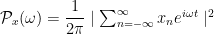
Rayleigh Power Statistic

The first thing we can do is simply check a simple, unbinned statistic for a given frequency, called the Rayleigh Power Statistic $S(\omega)$

$S(\omega)=\dfrac{1}{N}\left[\sum_{j=1}^{N}\cos(\omega t_{j})\right]^{2}+\left[\sum_{j=1}^{N}\sin(\omega t_{j})\right]^{2}$

By unbinned, we mean that we simply calculate the statistic for all data points without computing any histograms or using any kind of sampling.

What does this statistic measure? Suppose our times $t_{j}$ are uniformly distributed (i.e. werewolves come out at random). Then $S(\omega)=1$ We can compute a confidence of periodicity by using the statistic for a uniform distribution

$1-P(S(\omega)>k)=1-e^{-S(\omega)}$

For this data set, S=8167 for N=885, and $\omega=28$ days, our confidence is

$1-e^{-\dfrac{8167}{885}}=1-10^{-4}\gg 1$

So we have a very high confidence that werewolves do come out every 28 days.

What if we did not know the exact frequency $\omega$ ? No problem, we can just plot $S(\omega)$ vs $\omega$ and look for the peaks

So why not just do this? Where does this break down?

does not work for binned / sampled data
may perform poorly if the data is not evenly sampled?
not entirely clearly how to handle multiple frequencies

Traditional Spectral Analysis

Given a signal $x(t)$ , we are frequently interested in the power spectrum or energy signal density

$P(\omega)=\dfrac{1}{2\pi}\mid\int_{-\infty}^{\infty}x(t)e^{i\omega t}dt\mid^{2}=\dfrac{1}{2\pi}\mathcal{F}^{*}(\omega)\mathcal{F}(\omega)$

where $\mathcal{F}(\omega)$ is the continuous Fourier Transform of $f(t)$

We usually would approximate $\mathcal{F}(\omega)$ with the discrete-time Fourier Transform (DFT)

$\mathcal{P}_{x}(\omega)=\dfrac{1}{2\pi}\mid\sum_{n=-\infty}^{\infty}x_{n}e^{i\omega t}\mid^{2}$

although typically to obtain a good result we need to sample $x_{n}=x(t_{n})$ on equally spaced points $n$

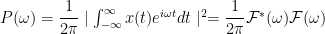
We then can now express the Periodogram

$P_{x}(\omega)=\dfrac{1}{N}\left[\left[\sum_{j}x_{j}\cos(\omega t_{j})\right]^{2}+\left[\sum_{j}x_{j}\sin(\omega t_{j})\right]^{2}\right]$

which is clearly the binned version of the Rayleigh Power Statistic, suitable for multiple frequencies.

We can express the Periodogram as the solution of the Least Squares (LS) optimization problem

$P_{x}(\omega)=\|\hat{\beta(\omega)}\|^{2}$ , where

$\hat{\beta(\omega)}=\min_{\beta(\omega)}\sum_{j=1}^{N}\|x(t_{j})-\beta e^{-i\omega t_{j}}\|^{2}$

Because our data is real, however, this expression is really

$\sum_{j=1}^{N}\|x(t_{j})-\beta(\omega)\cos(\omega t_{j}+\phi(\omega))\|^{2}+|\beta(\omega)|^{2}\sum_{j=1}^{N}\sin^{2}(\omega t_{j}+\phi(\omega))$

We see that LS problem includes a spurious term that does not depend on $x(t_{j})$ .

Consequently, in noisy time series, with uneven sampling, the standard Fourier approach will boost long-periodic noise. We need a different, more robust approach.

LSSA: Least Squares Spectral Analysis

What is LLSA? This approach is similar to the Periodogram above in that we formulate the problem as a LS optimization. We replace the spurious term above, however, by including an adjustable parameter $\tau$ in the cosine basis functions. Consider the following constrained minimization problem

$\min_{\beta,\phi}f_{\omega}(\beta,\phi)=\sum_{n=1}^{N}\left[x(t_{n})-\beta\cos(\omega(\tau-t_{n})+\phi)\right]^{2}$

where $\alpha\ge0$ and $\beta\in[0,2\pi]$ , and we constrain $\tau$ so that all the frequency components are mutually orthogonal at the sample times $t_{j}$

$\sum_{j=1}^{N}\cos(\omega(\tau-t_{j}))\sin(\omega(\tau-t_{j}))=0$

Rather than sample $x(t)$ on regular time intervals, and look at all frequency components, we will use regression and / or machine learning techniques to find the optimal $(\omega, \tau)$

We now can apply some old trigonometric identities. The constraint on $\tau$ can be expressed as

$\tan(2\omega\tau)=\dfrac{\sum_{n}\sin(2\omega t_{n})}{\sum_{n}\cos(2\omega t_{n})}$

and we can transform the overall function minimization to a constrained linear optimization problem using the identity

$\cos(x+y)=\cos(x)\cos(y)-\sin(x)\sin(y)$

This leads to

$cos(\omega(\tau-t_{n})+\phi)=cos(\omega(\tau-t_{n}))\cos(\phi)+sin(\omega(\tau-t_{n}))\sin(\phi)$

Let us now define the linear equation

$\mathbf{x}=\mathbf{A}\mathbf{\Phi}$ , where

$\mathbf{x}=\left[\begin{array}{c} x_{1}\\ x_{2}\\ \ldots\\ x_{N} \end{array}\right]$ , $\mathbf{A}=\left[\begin{array}{cc} \cos(\omega(\tau-t_{1})) & \sin\omega(\tau-t_{1}))\\ \cos(\omega(\tau-t_{2})) & \sin\omega(\tau-t_{2}))\\ \ldots & \ldots\\ \cos(\omega(\tau-t_{N})) & \sin\omega(\tau-t_{N})) \end{array}\right]$ , $\Phi=\left[\begin{array}{c} \beta\cos(\phi)\\ \beta\sin(\phi) \end{array}\right]$

This is now a linear constrained problem, normally solved by Ordinary Least Squares (OLS). We choose a quadratic loss function to illustrate, but, later, we will see we can also solve this problem as a Machine Learning optimization using an $L_{1}$ norm or any number of methods. Using OLS, we obtain

$\min f(\mathbf{\Phi})=\hat{\mathbf{\Phi}}=(\mathbf{A}^{t}\mathbf{A})^{-1}\mathbf{A}^{t}\mathbf{x}$

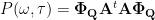
We can now express the Power Spectrum, or Periodgram, as

$P_{x}(\tau,\omega)=\dfrac{1}{N}\hat{\mathbf{\Phi}}^{t}\mathbf{A}^{t}\mathbf{A}\hat{\mathbf{\Phi}}$

Lomb-Scargle Periodgram

Without going into all the details yet, we can now express the spectral density $P_{x}(\omega)$ in closed form:

$P_{x}(\tau,\omega)=\dfrac{1}{2\sigma^{2}}\left(\dfrac{[\sum_{j}(x_{j}-\bar{x})\cos\omega(\tau-t_{j})]^{2}}{\sum_{j}X_{j}\cos^{2}\omega(\tau-t_{j})}\right)+\left(\dfrac{[\sum_{j}(x_{j}-\bar{x})\sin\omega(\tau-t_{j})]^{2}}{\sum_{j}X_{j}\sin^{2}\omega(\tau-t_{j})}\right)$

where $\bar{x}=\dfrac{1}{N}\sum^{N}_{i=1}x_{i}$ and $\sigma=\dfrac{1}{N-1}\sum^{N}_{i=1}(x_{i}-\bar{x})$ are the empirical mean and standard deviation, resp.

I will work out the proof soon

Extensions: Weighted Least Squares Spectral Analysis

When we have the covariance of our sample data, or some other model of the noise, we can include this into the OLS problem (see [4]). For example, we model the covariance at each frequency $\omega_{k}$ as

$\mathbf{Q_{k}}=\sum_{j\ne k}\mathbf{A}_{j}\mathbf{D}_{j}\mathbf{A^{t}}_{j}$ ,

where $\mathbf{D}_{k}$ is the diagonal matrix

$\mathbf{D}_{k}=\dfrac{a^{2}(\omega_{k})+b^{2}(\omega_{k})}{2}\left[\begin{array}{cc} 1 & 0\\ 0 & 1 \end{array}\right]$

We may plug in any estimate of the covariance $\mathbf{Q}$ to the OLS problem–as long as it is not ill-conditioned–yielding the new quadratic minimization functional

$\left[\mathbf{x}-\mathbf{A\Phi}\right]^{t}\mathbf{Q}\left[\mathbf{x}-\mathbf{A\Phi}\right]$

This leads to an improved expression for $\Phi$

$\mathbf{\Phi_{Q}}=(\mathbf{A}^{t}\mathbf{Q}^{-1}\mathbf{A})^{-1}\mathbf{A}^{t}\mathbf{Q}^{-1}\mathbf{x}$

but the Periodgram stil has the form of an expectation value of $\mathbf{A^{t}A}$

$P(\omega,\tau)=\mathbf{\Phi_{Q}}\mathbf{A}^{t}\mathbf{A}\mathbf{\Phi_{Q}}$

This should also lead to a similar, analytic expression for the Lomb-Scargle Periodgram [to come soon, see 11 and references therein]

Issues with LSSA

We note that neither FFT nor LLSA approaches are robust when the number of samples is small, when the sampling is uneven, or when the time between samples is longer than the period being sampled $(t_{i}-t_{i+1})\gg\dfrac{1}{\omega}$ See [11]. This case arises frequently in Astronomy, and needs to be handled using Machine Learning (or other) techniques such as a Maximum Likelihood Approach to the Rayleigh Power analysis (see [3]), or a Generalized Lomb-Scargle Periodogram [11]

Generalized Lomb-Scargle Periodogram: Weights and Offsets

There are several modern research papers [3],[4] (more to come) discussing the success and limitations of LLSA and its variants. Here we describe the variant provided in the AstroML package (below, to come)

Example: AstroML Package

The AstroML package [1] is very new and is built upon the very popular Scikits Learn Machine Learning library for Python. AstroML implements both the classical Lomb Scargle Periodogram and the Generalized version [11]. Here is an example

Here we have generated random data distributed around the function

$y=10.0+\sin(2\pi\omega t)$ , where $\omega=\dfrac{1}{0.3}$

and we compute the Periodogram for periods $\dfrac{1}{\omega}\in(0,1)$ . We see the Periodgram is quite noisy, but there is a dominant peak at $\dfrac{1}{\omega}=0.3$ .

Can we do better?

Machine Learning Alternatives

Just a hint of whats to come. Using traditional (odl school) machine learning / Kernel SVM techniques, one can model the covariances and/or other noise by using a non-linear, kernel-SVM (i.e. [9]) But we note that we can also recast the quadratic optimization problem as a linear programming problem, called Basis Pursuit

$\min_{\Phi}\|\mathbf{\Phi}\|_{1}$ subject to $\mathbf{x}=\mathbf{A}\mathbf{\Phi}$

or as a convex optimization, sometimes called Basis Pursuit Denoising

$\min_{\Phi}\|\mathbf{x}-\mathbf{A}\mathbf{\Phi}\|_{2}+\lambda\|\mathbf{\Phi}\|_{1}$

When would such approached be useful? The LSSA method would clearly be deficient when the OLS problem is pathological, or

$\int_{0}^{\omega_{max}}\mathbf{A}^{t}\mathbf{A}d\omega$

is ill-conditioned. (See the Appendix of reference [4] for more details).

In particular, when the LSSA problem is underdetermined, then we need advanced techniques. Which leads us to the next blog, where we will discuss the modern variants of these old AstroPhysics and Geophysics methods–called Compressed Sensing. Stay Tuned.