Causality, Correlation, and Brownian Motion

A recent question on Quora asked if machine learning could learn something from the Black Scholes model of Finance

http://www.quora.com/Machine-Learning/Can-we-learn-any-lessons-from-the-Black-Scholes-solution-to-pricing-risk-to-machine-learning-algorithms-for-personalization-recommendation-algorithms

I have been curious about this myself, but from a slightly different perspective, which I share here:

Introduction

There is a deep relation between statistical mechanics (stat mech) and machine learning (ML). From Exponential Families to Maximum Entropy to Deep Learning, stat mech is all over ML. Here, we are interested in distinguishing between causality and correlation, and the hope is we can learn from stat mech how to do this. We are motivated by a recent neuroscience paper [3] that suggests a new approach to Granger Causality via non-equilibirum statistical mechanics, specifically the Mori-Zwanzig Projection Operator formalism (see [6], my favorite reference, or just Google it). Also, very recent results [10] demonstrate that one can apply the Mori-Zwanzig formalism to a set of coupled stochastic variables like we see in Granger Causality and other time series models.

This is, however, pretty esoteric stuff, even if you have a PhD in Theoretical Chemistry like me. So before we dive in, in this post, we first look at a something ubiquitous in science: Brownian Motion

Causality in Statistical Mechanics

What is causality? Let’s pose it as a problem in time series analysis. Say we want to describe the dynamics of a system where one set of variables $X(t)$ dominate, but are driven, seemingly stochastically, by some other set of variables $Y(t)$ .

For example, $X$ might represent a particle floating in a viscous fluid $Y$ . As the particle moves, the fluid relaxes around it, leaving a slowly decaying trail.

So even though the particle $X$ appears to move randomly, its position at time $t+\delta t$ depends on both it’s entire history $X(t)$ and the history of the local surroundings $Y(t)$ . The more viscous, or stiff, the fluid is, the more the surroundings matter.

When can we say that $Y(t)$ causes $X(t)$ ?

The challenge in statistical mechanics is to decide when the particle is just random (i.e. a Brownian motion) and when the fluid is strongly affecting (i.e causing) a part of the dynamics.

Stochastic Problems in Astronomy and Physics

To get started, we need a some basic physics.

There is a classic review of Stochastic Problems in Astronomy and Physics [1] by the late Subrahmanyan Chandrasekhar, Nobel Laureate (Physics, 1983) and former head of the department of physics when I was a student at the University of Chicago.

I am a firm believer that every scientist should study and know the great works of the Nobel Laureates, so I strongly encourage the reader to dig deep [1] on their own–or to at least continue reading.

Chandrasekhar introduces the Langevin equation, and uses it to describe stochastic processes such as Random Walks and Mean-Reverting Walks (which are important for cointegration, but not discussed here)

Random Walks

When our particle is behaving randomly, and does not remember its history, we say it is undergoing a Random Walk. This is also known as Brownian Motion. Below we plot the path of several 1-D random walks over time. Notice that they all start at (0,0), but, over time, eventually diverge from each other.

Brownian motion is ubiquitous; it appears everywhere in Science. In Finance and Economics, it is described as a Wiener Process or with the Ito Stochastic Calculus. However, if we go old school, we can also describe the random walk using something familiar from high school calculus/physics. The model is

the Langevin equation:

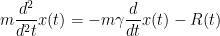
$m\dfrac{d^{2}}{d^{2}t}x(t)=-m\gamma\dfrac{d}{dt}x(t)-R(t)$

where $m$ is the mass, $m\gamma$ is a friction coefficient, and $R(t)$ represents the noise, interpreted as a random force.

What is this? We all know–or have least heard of–Newton’s famous equation

$F=ma$

Force equals mass times acceleration

Here, we flip this around, and have

$ma=F=F_f-F_R$

mass ( $m$ ) times acceleration $\dfrac{d^{2}}{d^{2}t}x(t)$ = Force

= Frictional Force ( $F_f$ ) minus Random Force ( $F_R$ )

where

the Frictional Force, $F_f=m\gamma\dfrac{d}{dt}x(t)$ , is a constant times velocity

and

the Random Force $F_R=R(t)$ is defined below

.
The random force represents the interactions of the particle with the solvent, which undergoes the thermal, random fluctuations (shown here)

We can not describe the random force with a dynamical equation, so, instead, we define $R(t)$ through it’s time-time auto-correlation functions

$\langle R(t)R(t)\rangle=0$

$\langle R(t_1)R(t_2)\rangle=2\pi_{R}G\delta(t_1-t_2)$

This correlation function is dot product in a Hilbert space; in fact it is a Kernel.

Here it is a constant; below we define a ‘memory Kernel’ that describes what is causing the random behavior (and also deals with the failures of the theory at short times)

Diffusion and the Einstein relation:

The particle $X$ moves around randomly; we say it diffuses. We identify a Diffusion constant, which is just the limit of average mean squared position, taken to very long times

$D=\underset{t\rightarrow\infty}{\lim}\dfrac{1}{2t}\langle (X(t)-X(t_{0}))^{2}\rangle$

It turns out the random force is not just any random force; it is intimately related to the other parameters in the equation. Einstein noted that the friction constant $m\gamma$ is related to the diffusion $D$ constant by

$D= \dfrac{k_{B}T}{m\gamma}$

where $k_{B}$ is Boltzman’s constant, and $T$ is the temperature.

With a little work (not shown here), we can also use the Einstein relation and our definition of the random force to express the Diffusion constant in terms of the time correlation of the velocity $u(t)$

$D=\int_{0}^{\infty}\langle u(t_{0})u(t_{0}+t)\rangle dt$ , where

This means that if the velocities are weakly correlated (over time), the surroundings drag on the particle, and it diffuses slower. On the other hand, when the velocities are strongly correlated, the particle does not feel the surroundings, and it diffuses faster.

Because the velocity platys such an important role, frequently we express the Langevin equation in terms of the velocity

$m\dfrac{d}{dt}u(t)=-m\gamma u(t)-R(t)$

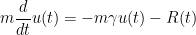
We can also express the velocity-velocity auto-correlation function as a simple exponential decay

$\langle u(t_{0})u(t_{0}+t)\rangle=\langle u^2\rangle\exp(-\gamma|t|)$

where

$\langle u^2\rangle=\dfrac{D}{\gamma}$

Not that our theory breaks down at short time scales because we expect the the velocity process to be stationary process. That is, we expect

$\langle u(t)\dfrac{d}{dt}u(t) \rangle=0$

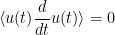
which is clearly not satisified.

On long timescales, the Langevin equation describes a mathematical Brownian motion, but on small timescales, the Langevin equation includes inertial effects that are not present in the Brownian description. These inertial affects can be very real, as shown above in the image of the pollen in the viscous fluid, and are corrected for below.

Also, we are considering systems that actually have velocities–this is important since we don’t usually think of pure stochastic processes, such as economic or financial time series, as having a well defined or instantaneous velocity.

Still, we are on the right track. We can relate the random forces directly to the macroscopic diffusion $D_{u}$ (in velocity space) through the correlation function of the random forces

$D_{u}\sim\int_{0}^{\infty}\langle R(t_{0})R(t_{0}+t)\rangle dt$

So we can determine how strongly the environment ’causes’ the dynamics by measuring an auto-correlation function of the random forces

We begin to see the link between correlation functions and causality. This is a direct example of

the Fluctuation-Dissipation theorem

<The fluctuation-dissipation theorem is a general result of statistical mechanics that quantifies the relation between the fluctuations in a system at equilibrium and its response to external perturbations. Basic examples include Brownian motion and Johnson–Nyqvist noise, but this phenomena also arise in non-equilibrium systems, and, perhaps, even in the neocortex.

Here, the same random forces that cause the erratic motion of a particle also causes drag. If something pulls the particle through the fluid, it feels this drag. The particle’s random motions and dissipative frictional forces have the same origin, or cause.

We can see this in 2 different ways:

We can apply an external force to the system and monitor the (linear) response
We can construct equilibrium velocity distribution and relate this to the self-diffusion

More generally, we can observe any external action $Y$ that “causes” $X$ to move by inferring the ‘equilibrium’ distribution, and computing the appropriate correlation function of the random forces; this is our link to causality.

What does this have to do with Machine Learning? Notice I said infer. For a general system, we will infer the so-called ‘equilibrium’ , or most likely, (Boltzman) distribution, using a variational method. Then we can directly evaluate the correlation functions (which are the partial derivatives of our calculated partition function). But first, we need a more robust Langevin equation to work with.

the Generalized Langevin Equation (GLE)

We can generalize the Langevin equation by redefining the Random Force through a different Kernel. Let

$\langle R(t_1)R(t_2)\rangle=\xi(t_1-t_2)$

where $\xi(t)$ is called the memory Kernel.

This gives rise to a Generalized Langevin Equation (GLE)

$\dfrac{d}{dt}u(t)=-\int_{t_0}^{t}\xi(t-t')u(t')dt+R(t)$

A typical application of the GLE in chemical physics to extend Brownian to describe the dynamics of a particle in a viscoelastic fluid (a fluid that is both thick and deformable); the memory Kernel gives rise to a generalized frictional force.

Some examples:

When memory effects matter, we have causality. Memory effects an appear in the velocity auto-correlation function (VACF) either through the presence of an oscillatory behavior or by means of slowly decreasing correlations [11]. In liquids, oscillations appear, for example, when particles are trapped, or caged, by their surroundings. And correlations slowly decrease in cases of anomalous diffusion, such as liquid-like defects [12]. Indeed, these effects arise all over physics, and, we suspect, in other systems as well. Only very recently, however, has the Mori-Zwanzig formalism been recognized as useful as a general mathematical tool for both optimal prediction [13], Markov Models [14], and Neuroscience [3]

Towards a Generalized Granger Causality

I would like to apply the GLE to problems in general machine learning. It would be necessary tointroduce a more abstract form of the GLE. We will then derive this GLE using the Mori-Zwanzig Projection Operator formalism from statistical mechanics.

It is then necessary how to infer the model parameters using variational techniques. Finally, we will demonstrate the relationship between Granger causality and a new measure that, we hope, will be more suitable in noisy, non-linear regimes. If time permits we will try to get to this

References

[1] Engle, Robert F., Granger, Clive W. J. (1987) “Co-integration and error correction: Representation, estimation and testing“, Econometrica, 55(2), 251–276.
[2] Stochastic Problems in Physics and Astronomy, Chandrasekhar, S. (The University of Chicago), Reviews of Modern Physics, vol. 15, Issue 1, pp. 1-89
[3] D.Hsu and M. Hsu (2009) Zwanzig-Mori projection operators and EEG dynamics: deriving a simple equation of motion
[4] Peter Hänggi, Fabio Marchesonia! Introduction: 100 years of Brownian motion
[5]http://web4.cs.ucl.ac.uk/staff/C.Bracegirdle/BayesianConditionalCointegration.php
[6] J.P. Hansen and I. R. McDonald (1986) , Theory of Simple Liquids
[7] http://www.dam.brown.edu/documents/Stinis_talk1.pdf
[8] Kubo, the Fluctuation-Dissipation Theorem
[9] Brownian motion: the Langevin model
[10] Jianhua Xing and K. S. Kim , Application of the projection operator formalism to non-Hamiltonian dynamics J. Chem. Phys. 134, 044132 (2011)
[13] Alexandre J. Chorin*, Ole H. Hald*, and Raz Kupferman, Optimal prediction and the MoriZwanzig representation of irreversible processes, PNAS (1999)
[14a] C. L. Beck, S. Lall§, T. Liang and M. West, Model reduction, optimal prediction, and the Mori-Zwanzig representation of Markov chains
[14b] Madhusudana Shashanka, A FAST ALGORITHM FOR DISCRETE HMM TRAINING USING OBSERVED TRANSITIONS
[15] Distinguishing cause from effect using observational data: methods and benchmarks (2104)
Youu assk to be a function of a competition for unmatched of the
about utile websites on the net. I’m loss to commend