?Deep Learning is presented as Energy-Based Learning
Indeed, we train a neural network by running BackProp, thereby minimizing the model error–which is like minimizing an Energy.
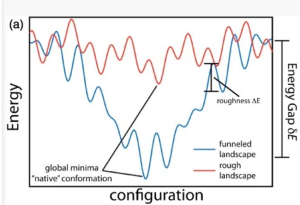
But what is this Energy ? Deep Learning (DL) Energy functions look nothing like a typical chemistry or physics Energy. Here, we have Free Energy landscapes, frequently which form funneled landscapes–a trade off between energetic and entropic effects.
And yet, some researchers, like LeCun, have even compared Neural Network Energies functions to spin glass Hamiltonians. To me, this seems off.
The confusion arises from assuming Deep Learning is a non-convex optimization problem that looks similar to the zero-Temperature Energy Landscapes from spin glass theory.
I present a different view. I believe Deep Learning is really optimizing an effective Free Energy function. And this has profound implications on Why Deep Learning Works.
This post will attempt to relate recent ideas in RBM inference to Backprop, and argue that Backprop is minimizing a dynamic, temperature dependent, ruggedly convex, effective Free Energy landscape.
This is a fairly long post, but at least is basic review. I try to present these ideas in a semi-pedagogic way, to the extent I can in a blog post, discussing both RBMs, MLPs, Free Energies, and all that entails.
BackProp
The Backprop algorithm lets us train a model directly on our data (X) by minimizing the predicted error 


Let’s write

where the error 

whereas for multi-class classification, we might minimize a categorical cross entropy

where 


Notice that 

Of course, we can adjust the network parameters, regularization, etc, to tune the architecture of the network. Although it appears that Understanding deep learning requires rethinking generalization.
At this point, many people say that BackProp leads to a complex, non-convex optimization problem; IMHO, this is naive.
It has been known for 20 years that Deep Learning does not suffer from local minima.
Anyone who thinks it does has never read a research paper or book on neural networks. So what we really would like to know is, Why does Deep Learning Scale ? Or, maybe, why does it work at all ?!
To implement Backprop, we take derivatives 

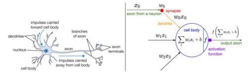
Layers and Activations
Let’s take a closer look at the layers and activations. Consider a simple 1 layer net:

The Hidden activations 


Indeed, the sigmoid activation function 

Moreover, Cowan pioneered using Statistical Mechanics to study the Neocortex.
And we will need a little Stat Mech to explain what our Energy functions are..but just a little.
Sigmoid Activations and Statistical Mechanics
While it seems we are simply proposing an arbitrary activation function, we can, in fact, derive the appearance of sigmoid activations–at least when performing inference on a single layer (mean field) Restricted Boltzmann Machine (RBM).
Hugo Larochelle has derived the sigmoid activations nicely for an RBM.
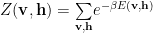
Given the (total) RBM Energy function

The log Energy is an un-normalized probability, such that

Where the normalization factor, Z, is an object from statistical mechanics called the (total) partition function Z
and 

Following Larochelle, we can factor 


We note that, this formulation was not obvious, and early work on RBMs used methods from statistical field theory to get this result.
RBM Training
We use 

CD has been a puzzling algorithm to understand. When first proposed, it was unclear what optimization problem is CD solving? Indeed, Hinton is to have said
Specifically, we run several epochs of:
- n steps of Gibbs sampling, or some other equilibration method, to set the neuron activations.
- some form of gradient descent
where
We will see below that we can cast RBM inference as directly minimizing a Free Energy–something that will prove very useful to related RBMs to MLPs
Energies and Activations
The sigmoid, and tanh, are an old-fashioned activation(s); today we may prefer to use ReLUs (and Leaky ReLUs).

The sigmoid itself was, at first, just an approximation to the heavyside step function used in neuron models. But the presence of sigmoid activations in the total Energy suggests, at least to me, that Deep Learning Energy functions are more than just random (Morse) functions.
RBMs are a special case of unsupervised nets that still use stochastic sampling. In supervised nets, like MLPs and CNNs (and in unsupervised Autoencoders like VAEs), we use Backprop. But the activations are not conditional probabilities. Let’s look in detail:
MLP outputs
Consider a MultiLayer Perceptron, with 1 Hidden layer, and 1 output node
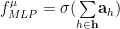
where 
and total MLP output

where 
If we add a second layer, we have the iterated layer output:

where 
The final MLP output function has a similar form:


So with a little bit of stat mech, we can derive the sigmoid activation function from a general energy function. And we have activations it in RBMs as well as MLPs.
So when we apply Backprop, what problem are we actually solving ?
Are we simply finding a minima on random high dimensional manifold ? Or can we say something more, given the special structure of these layers of activated energies ?
Backprop and Energy Minimization
To train an MLP, we run several epochs of Backprop. Backprop has 2 passes: forward and backward:

- Forward: Propagate the inputs
forward through the network, activating the neurons
- Backward: Propagate the errors
backward to compute the weight gradients

Each epoch usually runs small batches of inputs at time. (And we may need to normalize the inputs and control the variances. These details may be important for out analysis, and we will consider them in a later post).
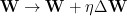
After each pass, we update the weights, using something like an SGD step (or Adam, RMSProp, etc)
For an MSE loss, we evaluate the partial derivatives over the Energy parameters 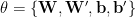
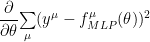
Backprop works by the chain rule, and given the special form of the activations, lets us transform the Energy derivatives into a sum of Energy gradients–layer by layer

I won’t go into the details here; there are 1000 blogs on BackProp today (which is amazing!). I will say…
Backprop couples the activation states of the neurons to the Energy parameter gradients through the cycle of forward-backward phases.
In a crude sense, Backprop resembles our more familiar RBM training procedure, where we equilibrate to set the activations, and run gradient descent to set the weights. Here, I show a direct connection, and derive the MLP functional form directly from an RBM.
From RBMs to MLPs
Discriminative (Supervised) RBMs
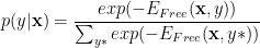
RBMs are unsupervised; MLPs are supervised. How can we connect them? Crudely, we can think of an MLP as a single layer RBM with a softmax tacked on the end. More rigorously, we can look at Generalized Discriminative RBMs, which solve the conditional probability directly, in terms of the Free Energies, cast in the soft-max form
So the question is, can we extract Free Energy for an MLP ?
the Backward Phase
I now consider the Backward phase, using the deterministic EMF RBM, as a starting point for understanding MLPs.
An earlier post discusses the EMF RBM, from the context of chemical physics. For a traditional machine learning perspective, see this thesis.
In some sense, this is kind-of obvious. And yet, I have not seen a clear presentation of the ideas in this way. I do rely upon new research, like the EMF RBM, although I also draw upon fundamental ideas from complex systems theory–something popular in my PhD studies, but which is perhaps ancient history now.
The goal is to relate RBMs, MLPs, and basic Stat Mech under single conceptual umbrella.
In the EMF approach, we see RBM inference as a sequence of deterministic annealing steps, from 1 quasi-equilibrium state to another, consisting of 2 steps for each epoch:
- Forward: equilibrate the neuron activations by minimizing the TAP Free Energy
- Backward: compute weight gradients of the TAP Free Energy
At the end of each epoch, we update the weights, with weight (temperature) constraints (i.e. reset the L1 or L2 norm). BTW, it may not obvious that weight regularization is like a Temperature control; I will address this in a later post.
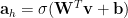
(1) The so-called Forward step solves a fixed point equation (which is similar in spirit to taking n steps of Gibbs sampling). This leads to a pair of coupled, recursion relations for the TAP magnetizations (or just nodes). Suppose we take t+1 iterations. Let us ignore the second order Onsager correction, and consider the mean field updates:
![h_{i}[t+1]\leftarrow\sigma\left[b_{i}+\underset{j}{\sum}w_{i,j}v_{j}[t+1]-\cdots\right]](https://s0.wp.com/latex.php?latex=h_%7Bi%7D%5Bt%2B1%5D%5Cleftarrow%5Csigma%5Cleft%5Bb_%7Bi%7D%2B%5Cunderset%7Bj%7D%7B%5Csum%7Dw_%7Bi%2Cj%7Dv_%7Bj%7D%5Bt%2B1%5D-%5Ccdots%5Cright%5D+&bg=ffffff&fg=%23000000&s=0&c=20201002)
![v_{i}[t+1]\leftarrow\sigma\left[a_{i}+\underset{j}{\sum}w_{i,j}h_{j}[t]-\cdots\right]](https://s0.wp.com/latex.php?latex=v_%7Bi%7D%5Bt%2B1%5D%5Cleftarrow%5Csigma%5Cleft%5Ba_%7Bi%7D%2B%5Cunderset%7Bj%7D%7B%5Csum%7Dw_%7Bi%2Cj%7Dh_%7Bj%7D%5Bt%5D-%5Ccdots%5Cright%5D+&bg=ffffff&fg=%23000000&s=0&c=20201002)
Because these are deterministic steps, we can express the ![h_{i}[t+1]\](https://s0.wp.com/latex.php?latex=h_%7Bi%7D%5Bt%2B1%5D%5C+&bg=ffffff&fg=%23000000&s=0&c=20201002)
![h_{i}[t]](https://s0.wp.com/latex.php?latex=h_%7Bi%7D%5Bt%5D+&bg=ffffff&fg=%23000000&s=0&c=20201002)
![\mathbf{h}[t+1]\leftarrow\sigma\left[\mathbf{b}+\mathbf{W}^{T}\sigma(\mathbf{b}+\mathbf{W}^{T}\mathbf{h}[t])\right]](https://s0.wp.com/latex.php?latex=%5Cmathbf%7Bh%7D%5Bt%2B1%5D%5Cleftarrow%5Csigma%5Cleft%5B%5Cmathbf%7Bb%7D%2B%5Cmathbf%7BW%7D%5E%7BT%7D%5Csigma%28%5Cmathbf%7Bb%7D%2B%5Cmathbf%7BW%7D%5E%7BT%7D%5Cmathbf%7Bh%7D%5Bt%5D%29%5Cright%5D+&bg=ffffff&fg=%23000000&s=0&c=20201002)
At the end of the recursion, we will have a forward pass that resembles a multi-layer MLP, but that shares weights and biases between layers:
![\mathbf{h}[t+1]\leftarrow\sigma\left[\mathbf{b}+\mathbf{W}^{T}\sigma(\mathbf{b}+\cdots\sigma(\mathbf{b}+\mathbf{v}\mathbf{W}^{T}))\right]](https://s0.wp.com/latex.php?latex=%5Cmathbf%7Bh%7D%5Bt%2B1%5D%5Cleftarrow%5Csigma%5Cleft%5B%5Cmathbf%7Bb%7D%2B%5Cmathbf%7BW%7D%5E%7BT%7D%5Csigma%28%5Cmathbf%7Bb%7D%2B%5Ccdots%5Csigma%28%5Cmathbf%7Bb%7D%2B%5Cmathbf%7Bv%7D%5Cmathbf%7BW%7D%5E%7BT%7D%29%29%5Cright%5D+&bg=ffffff&fg=%23000000&s=0&c=20201002)
We can now associate an n-layer MLP, with tied weights,

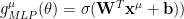
to an approximate (mean field) EMF RBM, with n fixed point iterations (ignoring the Onsager correction for now). Of course, an MLP is supervised, and an RBM is unsupervised, so we need to associate the RBM hidden nodes with the MLP output function at the last layer (
](https://s0.wp.com/latex.php?latex=g%5E%7B%5Cmu%7D_%7BMLP%7D%28%5Ctheta%29%3Dg%5E%7B%5Cmu%7D_%7BRBM%7D%28%5Ctheta%29%3D%5Cmathbf%7Bh%7D%5Bn%5D%28x%5E%7B%5Cmu%7D%29+&bg=ffffff&fg=%23000000&s=0&c=20201002)
This leads naturally to the following conjecture:
The EMF RBM and the BackProp Forward and Backward steps effectively do the same thing–minimize the Free Energy
Is this right ?
This is a work in progress
Formally, it is simple and compelling. Is it the whole story…probably not. It is merely an observation–food for thought.
So far, I have only removed the visible magnetizations ](https://s0.wp.com/latex.php?latex=%5Cmathbf%7Bv%7D%5Bn%5D%28x%5E%7B%5Cmu%7D%29+&bg=ffffff&fg=%23000000&s=0&c=20201002)
![\mathbf{v}[n],\mathbf{h}[n]= \mathbf{m_{v}},\mathbf{m_{h}}](https://s0.wp.com/latex.php?latex=%5Cmathbf%7Bv%7D%5Bn%5D%2C%5Cmathbf%7Bh%7D%5Bn%5D%3D+%5Cmathbf%7Bm_%7Bv%7D%7D%2C%5Cmathbf%7Bm_%7Bh%7D%7D++&bg=ffffff&fg=%23000000&s=0&c=20201002)
- unravel the network, like a variational auto encoder (VAE)
- replace the visible magnetizations with the true labels, and introduce the softax loss
The result itself should not be so surprising, since it has already been pointed out by Kingma and Welling, Auto-Encoding Variational Bayes, that a Bernoulli MLP is like a variational decoder. And, of course, VAEs can be formulated with BackProp.
Nore importantly, It is unclear how good the RBM EMF really is. Some followup studies indicate that second order is not as good as, say, AIS, for estimating the partition function. I have coded a python emf_rbm.py module using the scikit-learn interface, and testing is underway. I will blog this soon.
Note that the EMF RBM relies on the Legendre Transform, which is like a convex relaxation. Early results indicates that this does degrade the RBM solution compared to traditional Cd. Maybe BackProp may be effective relaxing the convexity constraint by, say, relaxing the condition that the weights are tied between layers.
Still, I hope this can provide some insight. And there are …
Implications
Free Energy is a first class concept in Statistical Mechanics. In machine learning, not always so much. It appears in much of Hinton’s work, and, as a starting point to deriving methods like Variational Auto Encoders and Probabilistic Programing.
But Free Energy minimization plays an important role in non-convex optimization as well. Free energies are a Boltzmann average of the zero-Temperature Energy landscape, and, therefore, convert a non-convex surface into something at least less non-convex.
Indeed, in one of the very first papers on mean field Boltzmann Machines (1987), it is noted that
“An important property of the effective [free] energy function E'(V,0,T) is that it has a smoother landscape than E(S) due to the extra terms. Hence, the probability of getting stuck in a local minima decreases.”
Moreover, in protein folding, we have even stronger effects, which can lead to a ruggedly convex, energy landscape. This arises when the system runs out of configurational entropy (S), and energetic effects (E) dominate.
Most importantly, we want to understand, when does Deep Learning generalize well, and when does it overtrain ?
LeCun has very recently pointed out that Deep Nets fail when they run out of configuration entropy–an argument I also have made from theoretical analysis using the Random Energy Model. So it is becoming more important to understand what the actual energy landscape of a deep net is, how to separate out the entropic and energetic terms, and how to characterize the configurational entropy.
Hopefully the small insight will be useful and lead to a further understanding of Why Deep Learning Works.

Dear Charles, thanks for this very interesting post! (and also for all the previous ones)
I agree in that there is a confusion in directly comparing NN Energy Functions to spin glass Hamiltonians, and that training a DNN is not the same as finding the minimum in a zero-temperature energy landscapes of a glass. But, even when we could talk about “effective Free Energies” as being a more accurate description of the Deep Learning funneled landscapes, don’t you think that the whole success of DNNs relies on the fact that there’s actually no-need to find a global minimum?
You can train your DNN with different training subsets and it should/will find different local minima (even of your free energy!!). The trick is that all this local minima are, to more or less extent, representative of the problem/characteristic you’re asking the DNN to learn. Their strength should rely in the redundancy of representations of such properties. Precisely that’s why, I think, people frequently find better statistical results when averaging over the predictions of separately trained NNs, instead of extensively training a single one.
Generalization lives in the tortuous repetitions of valleys and hills at a (relatively high) energy level, and not in a deep minimum of whatever energy or free energy one could define.
Luckily we did start “suffering” from local minima at some point in ML, that is where all the fun started !!!
LikeLike
I think the evidence for having ‘no global minima’ is anecdotal and a bit deceptive, and it is confused because of the lack of explicit Temperature. It was known 20 years ago that neural nets have high internal symmetries, (specifically that we observe replica symmetry breaking (RSB) simply due to symmetry). This feels more like a highly degenerate global minima than a simply having lots of low lying local minima. But more importantly, these are T=0 minima, and nets operate effectively at T=1. So even if we have lots of T=0 minima, the T=1 Free Energy is a Boltzmann average of all of them. Free Energy, just in itself, has the effect of ‘smoothing out’ a large number of local minima, providing a flatter, more convex landscape.
LikeLike
Thanks! I should probably read the cited literature before proceeding the discussion, specially if there are things very clearly know since 20 year ago that may not be obvious to me 🙂 . A priori, I definitely agree with a Free Energy smoothing out a large number of T=0 local minima, providing a flatter landscape. But it is not transparently clear to me that this should result in “a” convex landscape (with “more” convex I’m fine), therefore my comment above. Also, I think that any arguments about symmetries may get weaker if we talk about not-fully-connected neurons; and those nets, with lots of locality and higher frustration, are also learning. But of course these are very light words and not deep thoughts. Regards, and keep posting!
LikeLiked by 1 person
Well it is unclear what is going on . I suggested the idea of a rugged convex landscape because it is known from protein folding. The ideas was put forth by Wolynes, and he called it the spin glass of minimal frustration. In this context, the idea is that the convexification acts in the same way the retrieval phase acts in a Hopfield net. That is, there is a low lying energy state living below the spin glass transition which appears, and the learning occurs here–not in the glassy part. Since we don’t really know the phase diagram of these complex nets, it is simply easier to posit a low lying energy state that gets us out of the spin glass phase.
(This idea is also called topological trivialization by some spin glass people, and has been put forth by a group at UCLA. ALthough I did not know about this when I started these posts)
Like a protein, the energy landscape would not just be single peaked. This would be a very rigid structure with no chemical function. In other words, overtrained. Instead, the landscape probably has some deep local minim to provide some flexibility and motion. In other words, generalization.
Of course, we need an effective ‘dimension’ , or what chemists call a reaction coordinate, on which to drive. In protein folding, this is entropy: F=-TS. But we also have to consider T, and in Hopfield nets, the retrieval phase is a very low T phase, whereas in deep nets, we implicitly have T=1 . Then again, no effort is made to ensure T=1…it is just assumed. To that end, I think there is a more subtle reason connection to spin glasses that has been overlooked entirely. It is becoming clearly now that networks generalize well when they have an excess residual entropy.
For example, see LeCun’s very recent work on Entropy SGD, and I think Lecun is on the right track here, but, because they ignore the concept of Free Energy, they also ignore Temperature, and are trying to use ideas for T=0 spin glasses to a non-zero T phenomena.
I conjecture that this excess entropy in the network landscape is analogous to the excess configurational entropy of a supercooled glass. And in supercooled glasses, there is a phenomena known as the Adam-Gibbs relation, which basically says that the energy barriers go to infinity as the temperature is lowered. This is called the Entropy Crises, and it is seen even simple spin glass models like the Random Energy Model. (I discussed this in my online video ad MMDS) For a deep net, the effective Temperature is like like the norm of weights–in other words, the traditional weight-norm regularizer. Rugged convexification arises as a way to avoid the Entropy Crises. In other words, good generalization requires averaging over a some number of T=0 energy minima, thereby avoiding Entropy collapse.
LikeLike
Hi Charles,
I’ve always been ad-hoc by the ad-hoc setting of the thermodynamic temperature to unity in RBM’s (despite arguments concerning the minina and the energy landscape). I know its convenient, but for inference and temperature dependent tasks like annealing, the thermodynamic temperature (or its inverse) needs to be explicitly stated, since the partition function Z=Z(\beta, \lambda), where \lambda represents a configuration of weights and parameters. As an added consequence, the Crooks Fluctuation Theorem will also be satisfied. Further, on careful examination the inclusion of the inverse thermodynamic temperature will not effect the RBM properties, since the weights can be scaled as \beta\lambda \rightarrow \lambda.
LikeLike
In any deep net (RBM, MLP, CNN, …) , it is necessary to keep the weights from exploding. Weight norm regularization is an old method; batch norm the most recent. I have proposed that maintaining weight normalization is effectively like a temperature control. Recall that a true stat mech Energy is size extensive, and so just using an Energy based method should prevent the weight from exploding–in the limit of infinite training data. But implicit scaling does not control the Temperature. It has been now been confirmed that in RBMs (1) the effective T< 1 and (2) RBMs undergo an Entropy Crises as low T. As I proposed in the MDDS talk. However, it is true that it is unclear how the entropy crisis affects training and the RBM properties. The current idea is to assign an implicit T to the training data itself.
LikeLike