on Cheap Learning: Partition Functions and RBMs

“Why does deep and cheap learning work so well?“

This is the question posed by a recent article.  Deep Learning seems to require knowing the Partition Function–at least in old fashioned Restricted Boltzmann Machines (RBMs).

Here, I will discuss some aspects of this paper,  in the context of RBMs.

Preliminaries

We can use RBMs for unsupervised learning, as a clustering algorithm, for pretraining larger nets, and for generating sample data.   Mostly, however, RBMs are an older, toy model useful for understanding unsupervised Deep Learning.

RBMs

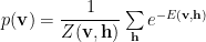
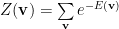
We define an RBM with an Energy Function

and it’s associated Partition Function

The joint probability is then

and the probability of  the visible units is computed by marginalizing over the hidden units

Note we also mean the probability of observing the data X={v}, given the weights W.

The Likelihood is just the log of the probability

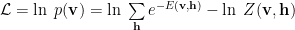
We can break this into 2 parts:

  is just the standard Free Energy

We call the clamped Free Energy

because it is like a Free Energy, but with the visible units clamped to the data X.

The clamped  is easy to evaluate in the RBM formalism, whereas is computationally intractable.

Knowing the is ‘like’ knowing the equilibrium distribution function, and methods like RBMs appear to approximate in some form or another.

RBM Training

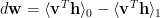
Training an RBM proceeds iteratively by approximating the Free Energies at each step,

and then updating W with a gradient step

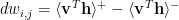
RBMs are usually trained via Contrastive Divergence (CD or PCD).  The Energy function, being quadratic, lets us readily factor Z using a mean field approximation, leading to simple expressions for the conditional probabilities

and the weight update rule

positive and negative phases

RBM codes may use the terminology of positive and negative phases:

:  The expectation is evaluated, or clamped, on the data.

:   The expectation  is to be evaluated on the prior distribution .  We also say is evaluated in the limit of infinite sampling, at the so-called equilibrium distribution.  But we don’t take the infinite limit.

CD approximates –effectively evaluating the (mean field) Free Energy —  by running only 1 (or more) steps of Gibbs Sampling.

So we may see

or, more generally, and in some code bases, something effectively like

Pseudocode is:

---

Initialize the positive   and negative

Run N iterations of:

Run 1 Step of Gibbs Sampling to get the negative  :

sample the hiddens given the (current) visibles: 

sample the visibles given the hiddens (above): 

Calculate the weight gradient:

Apply Weight decay or other regularization (optional):

Apply a momentum (optional):

Update the Weights:

---

Energy Renormalizations

What is Cheap about learning ?  A technical proof in the Appendix notes that

knowing the Partition function is not the same as knowing the underlying distribution .

This is because the Energy  can be rescaled, or renormalized, in many different ways, without changing .

This is a also key idea in Statistical Mechanics.

The Partition function is a generating function; we can write all the macroscopic, observable thermodynamic quantities as partial derivatives of .  And we can do this without knowing the exact distribution functions or energies–just their renormalized forms.

Of course, our W update rule is a derivative of 

The proof is technically straightforward, albeit a bit odd at first.

Matching Z(y) does not imply matching p(y)

Let’s start with the visible units .  Write

We now introduce the hidden units, , into the model, so that we have a new, joint probability distribution

and a new, Renormalized , partition function

Where RG means Renormalization Group.  We have already discussed that the general RBM approach resembles the Kadanoff Variational Renormalization Group (VRG) method, circa 1975. This new paper points out a small but important technical oversight made in the ML literature, namely that

having  does not imply

That is, just because we can estimate the Partition function well does not mean we know the probability distributions.

Why?   Define an arbitrary non-constant function and write

.

K is for Kadanoff RG Transform, and ln K is the normalization.

We can now write an joint Energy with the same Partition function as our RBM , but with completely different joint probability distributions.  Let

Notice what we are actually doing.  We use the K matrix to define the RBM joint Energy function.  In RBM theory, we restrict  to a quadratic form, and use variational procedure to learn the weights , thereby learning K.

In a VRG approach, we have the additional constraint that we restrict the form of K to satisfy constraints on it’s partition function, or, really, how the Energy function is normalized.  Hence the name ‘Renormalization.‘   This is similar, in spirit, but not necessarily in form, to how the RBM training regularizes the weights (above).

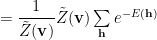
Write the total, or renormalized, Z as

Expanding the Energy function explicitly, we have

where the Kadanoff normalization factor appears now the denominator.

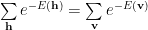
We can can break the double sum into sums over v and h

Identify in the numerator

which factors out, giving a very simple expression in h

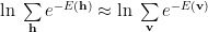
In the technical proof in the paper, the idea is that since h is just a dummy variable, we can replace h with v.  We have to be careful here since this seems to only applies to the case where we have the same number of hidden and visible units–a rare case.  In an earlier post on VRG, I explain more clearly how to construct an RG transform for RBMs.  Still,  the paper is presenting a counterargument for arguments sake, so, following the argument in the paper,  let’s say

This is like saying we constrain the Free Energy at each layer to be the same.

This is also another kind of Layer Normalization–a very popular method for modern Deep Learning methods these days.

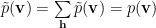
So, by construction, the renormalized and data Partition functions are identical

The goal of Renormalization Group theory is to redefine the Energy function on a difference scale, while retaining the macroscopic observables.

But , and apparently this has been misstated in some ML papers and books, the marginalized probabilities can be different !

To get the marginals, let’s integrate out only the h variables

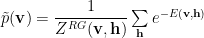
Looking above, we can write this in terms of K and its normalization

which implies

---

So what is cheap about deep learning ?

RBMs let us represent data using a smaller set of hidden features.  This is, effectively, Variational Renormalization Group algorithm,  in which we approximate the Partition function, at each step in the RBM learning procedure, without having to learn the underlying joining probability distribution.  And this is easier.  Cheaper.

In other words, Deep Learning is not Statistics.  It is more like Statistical Mechanics.  

And the hope is that we can learn from this old scientific field — which is foundational to chemistry and physics — to improve our deep learning models.

Post-Post Comments

Shortly after this paper came out, Comment on “Why does deep and cheap learning work so well?”that the proof in the Appended is indeed wrong–as I suspected and pointed out above.

It is noted that the point of the RG theory is to preserve the Free Energy form one layer to another, and, in VRG, this is expressed as a trace condition on the Transfer operator

where

It is, however, technically possible to preserve the Free Energy and not preserve the trace condition.  Indeed, because is not-constant, thereby violating the trace condition.

From this bloggers perspective, the idea of preserving Free Energy, via either a trace condition, or, say, by layer normalization, is the import point.  And this may mean to only approximately satisfy the trace condition.

In Quantum Chemistry, there is a similar requirement, referred to as a Size-Consistency and/ or Size-Extensivity condition.  And these requirements proven essential to obtaining highly accurate, ab initio solutions of the molecular electronic Schrodinger equation–whether implemented exactly or approximately.

And, I suspect, a similar argument, at least in spirit if not in proof, is at play in Deep Learning.

Please chime in our my YouTube Community Channel

see also: https://m.reddit.com/r/MachineLearning/comments/4zbr2k/what_is_your_opinion_why_is_the_concept_of/)