Deep Learning is amazing. But why is Deep Learning so successful? Is Deep Learning just old-school Neural Networks on modern hardware? Is it just that we have so much data now the methods work better? Is Deep Learning just a really good at finding features. Researchers are working hard to sort this out.
Recently it has been shown that [1]
Unsupervised Deep Learning implements the Kadanoff Real Space Variational Renormalization Group (1975)
This means the success of Deep Learning is intimately related to some very deep and subtle ideas from Theoretical Physics. In this post we examine this.
Unsupervised Deep Learning: AutoEncoder Flow Map
An AutoEncoder is a Unsupervised Deep Learning algorithm that learns how to represent an complex image or other data structure 
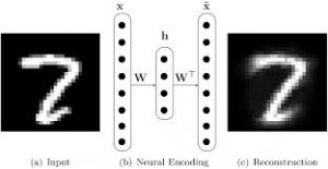
The simplest Neural Encoder is a Restricted Boltzman Machine (RBM). An RBM is non-linear, recursive, lossy function 


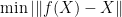
The RBM is learned by selecting the optimal parameters 
RBMs and other Deep Learning algos are formulated using classical Statistical Mechanics. And that is where it gets interesting!
Multi Scale Feature Learning
In machine learning (ML), we map (visible) data into (hidden) features

The hidden units discover features at a coarser grain level of scale

With RBMs, when features are complex, we may stack them into a Deep Belief Network (DBM), so that we can learn at different levels of scale

and leads to multi-scale features in each layer

Deep Belief Networks are a Theory of Unsupervised MultiScale Feature Learning
Fixed Points and Flow Maps
We call

eIf we apply the flow map to the data repeatedly, (we hope) it converges to a fixed point

Notice that we usually expect to apply the same map each time 
Example: Linear Flow Map
The simplest example of a flow map is the simple linear map

so that

where C is a non-negative, low rank matrix

We have seen this before: this leads to a Convex form of NonNegative Matrix Factorization NMF
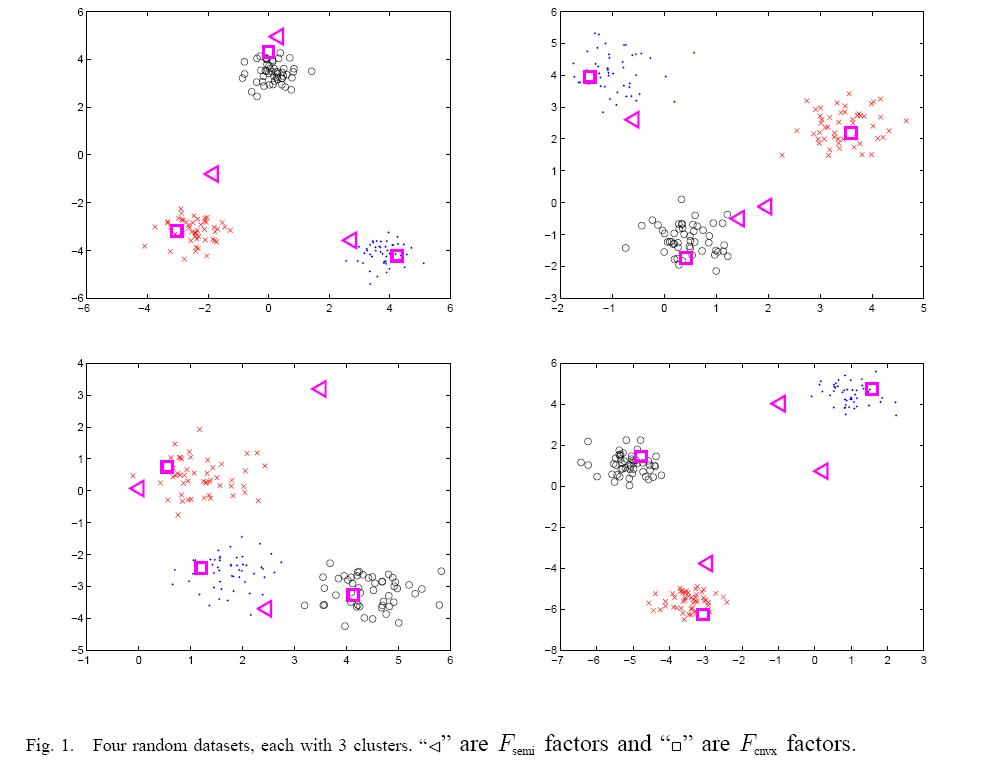
Convex NMF applies when we can specify the feature space and where the data naturally clusters. Here, there are a few instances that are archetypes that define the convex hull of the data.

Amazingly, many clustering problems are provably convex–but that’s a story for another post.
Example: Manifold Learning
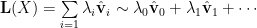
Near a fixed point, we commonly approximate the flow map by a linear operator

This lets us capture the structure of the true data manifold, and is usually described by the low lying eigen-spectra of
In the same spirit, Semi & Unsupervised Manifold Learning, we model the data using a Laplacian operator 


These methods include Spectral Clustering, Manifold Regularization , Laplacian SVM, etc. Note that manifold learning methods, like the Manifold Tanget Classifier, employ Contractive Auto Encoders and use several scale parameters to capture the local structure of the data manifold.
The Renormalization Group
In chemistry and physics, we frequently encounter problems that require a multi-scale description. We need this for critical points and phase transitions, for natural crashes like earthquakes and avalanches, for polymers and other macromolecules, for strongly correlated electronic systems, for quantum field theory, and, now, for Deep Learning.
A unifying idea across these systems is the Renormalization Group (RG) Theory.
Renormalization Group Theory is both a conceptual framework on how to think about physics on multiple scales as well as a technical & computational problem solving tool.
 Ken Wilson won the 1982 Nobel Prize in Physics for the development and application of his Momentum Space RG theory to phase transitions.
We used RG theory to model the recent BitCoin crash as a phase transition.
Wilson invented modern multi-scale modeling; the so-called Wilson Basis was an early form of Wavelets. Wilson was also a big advocate of using supercomputers for solving problems. Being a Nobel Laureate, he had great success promoting scientific computing. It was thanks to him I had access to a Cray Y-MP when I was in high school because he was a professor at my undergrad, The Ohio State University.
Here is the idea. Consider a feature map which transforms the data

The RG theory requires that the Free Energy 
the Free Energy is both Size-Extensive and Scale Invariant near a Critical Point
This is not obvious — but it is essential to both having a conceptual understanding of complex, multi scale phenomena, and it is necessary to obtain very highly accurate numerical calculations. In fact, being size extensive and/or size consistent is absolutely necessary for highly accurate quantum chemistry calculations of strongly correlated systems. So it is pretty amazing but perhaps not surprising that this is necessary for large scale deep learning calculations also!
The Fundamental Renormalization Group Equation (RGE)

If we (can) apply the same map,
Many RG formulations both approximate the exact RGE and/or only include relevant variables. To describe a multiscale system, it is essential to distinguish between these relevant and irrelevant variables.
Example: Linear Rescaling
Let’s say the feature map is a simple linear rescaling

We can obtain a very elegant, approximate RG solution where F(x) obeys a complex (or log-periodic) power law.

This behavior is thought to characterize Per-Bak style Self-Organized Criticality (SOC), which appears in many natural systems–and perhaps even in the brain itself. Which leads to the argument that perhaps Deep Learning and Real Learning work so well because they operate like a system just near a phase transition–also known as the Sand Pile Model--operating at a state between order and chaos.
the Kadanoff Variational Renormalization Group (1975)
 Leo Kadanoff, now at the University of Chicago, invented some of the early ideas in Renormalization Group. He is most famous for the Real Space formulation of RG, sometimes called the Block Spin approach. He also developed an alternative approach, called the Variational Renormalization Group (VRG, 1975), which is, remarkably, what Unsupervised RBMs are implementing!
Let’s consider a traditional Neural Network–a Hopfield Associative Memory (HAM). This is also known as an Ising model or a Spin Glass in statistical physics.
An HAM consists of only visible units; it stores memories explicitly and directly in them:
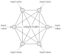
We specify the Energy — called the Hamiltonian 
The Hopfield model has only single 

A general Hamiltonian might have many-body, multi-scale interactions:

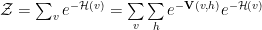
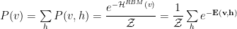
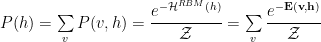
The Partition Function is given as

And the Free Energy is

The idea was to mimic how our neurons were thought to store memories–although perhaps our neurons do not even do this.
Either way, Hopfield Neural Networks have many problems; most notably they may learn spurious patterns that never appeared in the training set. So they are pretty bad memories.
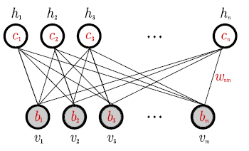
Hinton created the modern RBM to overcome the problems of the Hopfield model. He used hidden units to represent the features in the data–not to memorize the data examples directly.

An RBM is specified Energy function for both the visible and hidden units

This also defines joint probability of simultaenously observing a configuration of hidden and visible spins
which is learned variationally, by minimizing the reconstruction error…or the cross entropy (KL divergence), plus some regularization (Dropout), using Greedy layer-wise unsupervised training, with the Contrastive Divergence (CD or PCD) algo, …
The specific details of an RBM Energy are not addressed by these general concepts; these details do not affect these arguments–although clearly they matter in practice !
It turns out that
Introducing Hidden Units in a Neural Network is a Scale Renormalization.
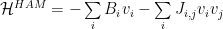
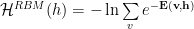
When changing scale, we obtain an Effective Hamiltonian 

or, in operator form
![\tilde{\mathcal{H}}(h)=\mathbb{R}[\mathcal{H}(v)]](https://s0.wp.com/latex.php?latex=%5Ctilde%7B%5Cmathcal%7BH%7D%7D%28h%29%3D%5Cmathbb%7BR%7D%5B%5Cmathcal%7BH%7D%28v%29%5D+&bg=%23ffffff&fg=%23000000&s=0&c=20201002)
This Effective Hamiltonian is not specified explicitly, but we know it can take the general form (of a spin funnel, actually)

The RG transform preservers the Free Energy (when properly rescaled):

where
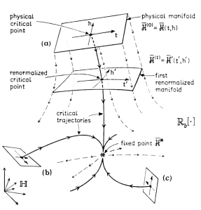
Critical Trajectories and Renormalized Manifolds
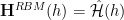
The RG theory provides a way to iteratively update, or renormalize, the system Hamiltonian. Each time we add a layer of hidden units (h1, h2, …), we have
![\mathcal{H}^{RG}(\mathbf{v},\mathbf{h1})=\mathbb{R}[\mathcal{H}(\mathbf{v})]](https://s0.wp.com/latex.php?latex=%5Cmathcal%7BH%7D%5E%7BRG%7D%28%5Cmathbf%7Bv%7D%2C%5Cmathbf%7Bh1%7D%29%3D%5Cmathbb%7BR%7D%5B%5Cmathcal%7BH%7D%28%5Cmathbf%7Bv%7D%29%5D+&bg=%23ffffff&fg=%23000000&s=0&c=20201002)
![\mathcal{H}^{RG}(\mathbf{v},\mathbf{h1},\mathbf{h2})=\mathbb{R}[\mathbb{R}[\mathcal{H}(\mathbf{v})]](https://s0.wp.com/latex.php?latex=%5Cmathcal%7BH%7D%5E%7BRG%7D%28%5Cmathbf%7Bv%7D%2C%5Cmathbf%7Bh1%7D%2C%5Cmathbf%7Bh2%7D%29%3D%5Cmathbb%7BR%7D%5B%5Cmathbb%7BR%7D%5B%5Cmathcal%7BH%7D%28%5Cmathbf%7Bv%7D%29%5D+&bg=%23ffffff&fg=%23000000&s=0&c=20201002)

We imagine that the flow map is attracted to a Critical Trajectory which naturally leads the algorithm to the fixed point. At each step, when we apply another RG transform, we obtain a new, Renormalized Manifold, each one closer to the optimal data manifold.
Conceptually, the RG flow map is most useful when applied to critical phenomena–physical systems and/or simple models that undergo a phase transition. And, as importantly, the small changes in the data should ‘wash away’ as noise and not affect the macroscopic / critical phenomena. Many systems–but not all–display this.
Where Hopfield Nets fail to be useful here, RBMs and Deep Learning systems shine.
We now show that these RG transformations are achieved by stacking RBMs and solving the RBM inference problem!
Kadanoff’s Variational Renormalization Group
As in many physics problems, we break the modeling problem into two parts: one we know how to solve, and one we need to guess.
- we know the Hamiltonian at the most fine grained level of scale
- we seek the correlation
that couples to the next level scale

The joint Hamiltonian, or Energy function, is then given by

The Correlation V(v,h) is defined so that the partition function 

This gives us
(Sometimes the Correlation V is called a Transfer Operator T, where V(v,h)=-T(v,h) )
We may now define a renormalized effective Hamilonian 
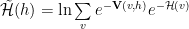
so that we may write

Because the partition function does not change, the Exact RGE preserves the Free Energy (up to a scale change, we we subsume into

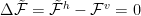
We generally can not solve the exact RGE–but we can try to minimize this Free Energy difference.
What Kadanoff showed, way back in 1975, is that we can accurately approximate the Exact Renormalization Group Equation by finding a lower bound using this formalism
Deep learning appears to be a real-space variational RG technique, specifically applicable to very complex, inhomogenous systems where the detailed scale transformations have to be learned from the data
RBMs expressed using Variational RG
We will now show how to express RBMs using the VRG formalism and provide some intuition
In an RBM, we simply want to learn the Energy function directly; we don’t specify the Hamiltonian for the visible or hidden units explicitly, like we would in physics. The RBM Energy is just

We identify the Hamiltonian for the hidden units as the Renormalized Effective Hamiltonian from the VRG theory
RBM Hamiltonians / Marginal Probabilities
To obtain RBM Hamiltonians for just the visible 


and
Training RBMs
To train an RBM, we apply Contrastive Divergence (CD), or, perhaps today, Persistent Contrastive Divergence (PCD). We can kindof think of this as slowly approximating

In practice, however, RBM training minimizes the associated Free Energy difference 
In the “Practical Guide to Training Restricted Boltzmann Machines”, Hinton explains how to train an RBM (circa 2011). Section 6 addresses “Monitoring the overfitting”
“it is possible to directly monitor the overfitting by comparing the free energies of training data and held out validation data…If the model is not overfitting at all, the average free energy should be about the same on training and validation data”
Other Objective Functions
Modern variants of Real Space VRG are not “‘forced’ to minimize the global free energy” and have attempted other approaches such as Tensor-SVD Renormalization. Likeswise, some RBM / DBM approaches do likewise may minimize a different objective.
In some methods, we minimize the KL Divergence; this has a very natural analog in VRG language [1].
Why Deep Learning Works: Lessons from Theoretical Physics
The Renormalization Group Theory provides new insights as to why Deep Learning works so amazingly well. It is not, however, a complete theory. Rather, it is framework for beginning to understand what is an incredibly powerful, modern, applied tool. Enjoy!
References
[1] An exact mapping between the Variational Renormalization Group and Deep Learning, 2014
[2] Variational Approximations for Renormalization Group Transformations, 1976
[3] A Common Logic to Seeing Cats and Cosmos
[4] WHY DOES UNSUPERVISED DEEP LEARNING WORK? – A PERSPECTIVE FROM GROUP THEORY, 2015
[5] A Fundamental Theory to Model the Mind
[6] A Practical Guide to Training Restricted Boltzmann Machines, 2010
[7] On the importance of initialization and momentum in deep learning, 2013
[8] Dropout: A Simple Way to Prevent Neural Networks from Overfitting, 2014
[9] Ken Wilson, A Scientific Appreciation
[10] http://www-math.unice.fr/~patras/CargeseConference/ACQFT09_JZinnJustin.pdf
[11] Training Products of Experts by Minimizing Contrastive Divergence, 2002
[12] Training Restricted Boltzmann Machines using Approximations to the Likelihood Gradient, 2008
[13] http://www.nonlin-processes-geophys.net/3/102/1996/npg-3-102-1996.pdf
[14] THE RENORMALIZATION GROUP AND CRITICAL PHENOMENA, Ken Wilson Nobel Prize Lecture
[15] Scaling, universality, and renormalization: Three pillars of modern critical phenomena
[16] The Potential Energy of an Autoencoder, 2014
[17] Contractive Auto-Encoders: Explicit Invariance During Feature Extraction, 2011

Reblogged this on Do not stop thinking.
LikeLike
Reblogged this on Importantish.
LikeLike
(Let me prephrase that I am not sure if LaTeX / MathJax works in the comment section; I am just going to type it out so that you might copy-paste the equations into your post, in case my stuff is actually correct….):
You write for the “renormalized Hamiltonian” acting only on the hidden units:
\[ \tilde{\mathcal{H}}(v) = \sum_v \mathrm{e}^{-V(v,h) – \mathcal{H}(v)} \]
I believe, \(\tilde{\mathcal{H}}(v)\) is a typo and should be \(\tilde{\mathcal{H}}(h)\) (since we are integrating out the visible degrees of freedom).
Next, I wonder about the definition as such: in order for the partition function to be unchanged, shouldn’t the definition of \(\tilde{\mathcal{H}}(h)\) involve a logarithm? I.e.:
\[\tilde{\mathcal{H}}(h) \rightarrow \tilde{\mathcal{H}}(h) = \log \sum_v \mathrm{e}^{-V(v,h) – \mathcal{H}(v)}\]
This way we exactly get \( \mathrm{e}^{\tilde{\mathcal{H}}(h)} = \sum_v \mathrm{e}^{-V(v,h) – \mathcal{H}(v) \), and we can plug this directly into the partition function.
LikeLike
thanks for reading
those are typos
you are awesome !
LikeLike
This is great! I was asking around a couple months ago for some kind of explanation of the connection.
I’ll read up on this!
LikeLike
It seems however that deep learning networks do not have the most essential property of such a physical system. The hidden states in a sandpile are not some “higher-level” sand grains. They are macroscopic observables. A deep learning network, however, does explicitly represent the hidden states by neurons. I blame it on its non-recursive structure.
What I don’t understand is how the “full connectivity” between a layer and its hidden representation (the next layer) does represent the locality as in block renormalization. It is fully connected, so why would it only get rid of local correlations? The coupling in spin lattices is normally only between neighbours.
The renormalization group has a fixed point when we do the mapping an infinite number of times. Does this mean the network converges only with an infinite number of layers? I think such a “rolled out” version is hardly exhibiting “self-organized criticality”, that is, if scientist would agree on a definition of SOC :-).
IMHO a single recurrent layer can exhibit renomalization group properties in a more fundamental way.
Or am I misunderstanding everything here? Forgive my ignorance. Some explanations would be really appreciated!
LikeLike
Thanks for stopping by and reading my post
I think, as with lots of complexity theory, we rely a lot upon analogy. Recall that here we are trying to learn the parameters of the network / Ising model, so we are doing a kind of inverse statistical mechanics, as opposed to proposing a symmetric, uniform random distribution of couplings. It is known that , during the learning phase of an RBM, it is necessary to either run a few steps of CD or run PCD. That is, 1 step of CD, then 3 steps of CD, etc. This suggests to me that the system is evolving along something akin to a flow map, and that we can only invert the equations exactly when we are near the critical point. As we add more layers, we are effectively adding 1 more iteration of the RG group, as opposed to solving it exactly for all iterations.
So, as in the picture, there are 2 lines of flow: the progress learning, and the number of RG transforms applied.
Why do we only keep local interactions? Well, to me this s analogous to the electron correlation problem in quantum chemistry. We usually start with some Hartree Fock (i.e. mean field, product of experts) solution, and then add in correlations vi some perturbation / renormalization steps. The RBM model is an analogous products of experts solution, which we can solve easily. Does this mean we have to remove all local correlations–well there are lots of details necessary to prevent the system from collapsing. Indeed, I suspect that the RBM state, along with regularization and dropout, prevent the model from collapsing into a spin glass ground state. Here, I am at odds with LeCun, who thinks that the reason the Deep Learning systems work is exactly because they are a spin glass. Of course, removing these connections may simply be that there are too many of them and the system overtrains, spin glass or not.
IMHO, this needs more investigation. And I agree with the RNN comment
Finally, I want to pose the following question. Suppose we run an unsupervised clustering algorithms on some data, twice but w/ different parameters. Which set produces better clusters? Most algos have no answer, and this is a central, very practical problem in basic ML. Here, I think we could say the better set is the one that more closely conserves the free energy between layers. This is a property of the RG approach, or, in quantum chemistry, is related to what we call size-consistencey. This allows us to search a massive space of parameters — which is impossible for general non-convex searches. and I suspect this is a key idea as to why these methods perform so well.
LikeLike
Maybe I am a bit slow. But to apply block renormalization in the network (N-dimensional spin lattice):
* what are the neighbours of a node?
* what exactly is the decimation step?
I don’t understand the exact equivalence.
Regarding number of clusters, I’m normally following a Bayesian approach and would just consider a prior on the distribution of items over clusters, using something like a Dirichlet Process or Pitman-Yor, etc. If this information is not available, I can understand that you’ll have to use something that just relates distributions over states on two different levels of abstraction. Free energy of some kind of quantity is probably involved. 🙂
With respect to dropout I recommend “Dropout as a Bayesian Approximation: Insights and Applications” by Gal and Ghahramani. The relation with Gaussian Processes promises a dropout method for RNNs as well!
LikeLike
My late (2 years later) opinion on this: “* what are the neighbours of a node?” and “The problem is that the local connection should be there from the start.”.
It is not very clear that you need a strong definition of neighbours or locality. In physics this happens in disordered media for instance, in which you can have long range interactions because of the disorder. In this situation the locality does not mean much. Indeed if you construct clusters from spins that are spatially close they may not be interacting because of the disorder. Therefore your decimation process is locally equivalent to a decimation on a free non interacting model (which is not interesting). It is probably much more interestng to cluster together degree of freedom (dof) that are strongly interacting (eventhough they may be spatially far). Actually the local clustering is natural in local field theory (FT), but it is not obvious that it is needed. Actually it is not, at least in some cases I know about.
You could also consider Ising model on arbitrary graphs instead of a lattice and you still expect that renormalization works (it probably exists in the physics literature already, I know about the random planar maps case, the random non-planar case should exist as well, but the key word ‘random’ simplifies things a lot here).
Then if you follow my point above I would say that you can create ‘natural’ clusters of neighbours by looking at the edge weight magnitudes between layers. Lets say you have a layer i with 6 nodes and a layer i+1 with 3 nodes. Then say that nodes 1,2,3 of the ith layer have all high values of their weight magnitude towards node 1 of layer i+1, while nodes 4,5,6 of layer i have only very small (in magnitude) weights to node 1 of layer i+1. Then I would say that node 1,2,3 are clustered together and decimated by node 1 of layer i (because the magnitude of their weights towards the same node 1 are comparable in magnitude). Of course this would mean that some dof will be taken into account more than once in the decimation process while some dof will simply be forgotten. But intuitively I feel that it still could lead to a decent renormalization process (as long as the over\under-counting of dof is not too big, which means, I guess, that the weight matrix has to be neither too sparse nor too diffuse, so this relates to the choice of regularization of the NN. Strangely enough this makes me think about another picture in Wetterich-like renormalization).
Dropout in this context might be seen as a way of averaging different renormalization processes in order to enhance the probability of following a ‘universal flow trajectory’ that leads to an interesting fixed point .
But anyway, I still think this is only a very very vague connection to renormalization and these ideas should be investigated rigorously before claiming that NN are just performing renormalization (that is why the ‘exact mapping’ paper title choice looks like pure marketing to me).
LikeLike
The main contribution is that VRG approach by Kadanoff resembles an RBM or DBM.
I agree, there is no discussion about decimation, or the fact that these are mean field methods.
I make a simple observation about free-energy based deep nets, like RBMs and DBMs.
The idea is, when defining the total Free Energy, one should also consider the constraint on the correlation operator V(h,v) such that the partition function is not changed. That is, in an RBM or DBM, we can try to define a free energy per layer, and ensure that the layer free energies are conserved. I don’t think anyone has tried this. The closest thing I know to this is bath normalization (for supervised nets). I don’t know if they are the same.
LikeLike
1. the variational approach is different from the real space decimation approach; roughly, the decimation step is like adding a layer
2. what happened to the local connections ? in a Hopfield network, all nodes are visible. In an RBM, there visible nodes are connected through the hidden layer, but not directly. This does not mean the visible nodes are not connected. To see this, one would need to construct an effective Hamiltonian for the visible nodes that includes the hidden interactions as renormalized visible-visible interactions.
Thanks for the references on the bayesian methods–ill check them out.
LikeLike
1. In a sandpile this would mean that all grains are connected to all grains on the next level. Then there would be some process (an inference process in the network). And magically, there will be local structure arising. And hey, this is a variational approximation to real-space renormalization. That’s not how it works… In the words of the authors: “Surprisingly, this local block spin structure emerges from the training process, suggesting the DNN is self-organizing to implement block spin renormalization”. I bet if you use textures as input of the network there is no such local structure arising. And local structure could just as well have originated from the ad-hoc applied L1 regularization (see Appendix).
2. The problem is that the local connection should be there from the start. In normal renormalization group approaches large-scale correlations arise from short-scale correlations. Here the authors start with a restricted Boltzmann machine: hidden nodes are connected to all visible nodes. Newman and Watts have a renormalization group on a small-world network, but there the decimation operator is quite different. That’s why I asked what the exact decimation operator is. It is not in the paper, because it “emerges”. Miracle!
If I may, let me ask one more detailed question…
Equation 10, where is it actually used? Does the form of the network matter? I think if Eq. 10 would describe a black hole the rest would still stand, saying something very trivial. Namely that you can minimize the KL divergence between two layers in a network and that this can be described by Hamiltonians.
LikeLike
The form of the network — eg 10 — is not used in this derivation.
I personally don’t know how important this is.
I have a more of experience with large scale perturbative ‘renormalization’ techniques from quantum chemistry. To me, these systems more resemble machine learning systems since they are large but finite, highly non-uniform, and not amenable to exact solutions. Also, it is not clear that we can apply RG arguments directly since we have to consider that we are learning the weights (i.e the H-V couplings)
I would say that
1. does eq 10 really matter? This is a key question
Well, generally speaking, it is necessary to choose the correct zeroth order description, but also one that is amenable to computational exploration
the RBM is also convenient computationally and it is unclear to me if similar results could be obtain using a formalism that includes local correlations directly. Perhaps adding them early on would improve the learning rate, or perhaps they would screw it up and cause it to overtrain?
2. removing local interactions may be corrected , in many situations, by simply to run higher order calculations.
if H= Ho+V , we can pick Ho to be diagonal in a localized basis (so there are no local interactions), and the off-diagonal parts just go into the interaction V.
that is, as we learn the weights, i kinda assumed the RBM would be a mean field approximation and effectively include the local interactions this way
I used this method (mean-field like H0, without overlap between sites) when computing effective Hamiltonians for pi-electron systems
http://pubs.acs.org/doi/abs/10.1021/jp960617w?journalCode=jpchax
in an RG formalism this might mean taking a higher order approximation to the RG operator. In a DBN, this might mean adding more layers, running more epochs, etc.
3. (1,2) , plus the danger of overtraining, implies to me that we may not / probably do not want to solve an Exact RGE
Exact RG calculations can lead to funny behavior and the details of the system do matter See, for example
http://journals.aps.org/prb/abstract/10.1103/PhysRevB.15.4476
so using variational RG is fine
So I’m not sure what the beef is here? Or if this was a beef?
It is true that the comparison is only partial; we set up the VRG formalism and apply the idea of finding a lower bound. What we can not do here is analyze the fixed point of the RG flow map using any kind of analytic theory. Moreover, this is the other ‘reaction coordinate’, which is the learning process. so it’s not like we are applying the RG transform, or the decimations, iteratively over and over–we have maybe a few layers, which corresponds to a few ‘decimations’ (if you want to call them that), and the ‘flow map’ is really saying that we are trying to find the Hamiltonian that is somewhere near the fixed point of the learning process, and not the fixed point of the RG iterations. Instead, what I assume is that when we get close to the the learned solution, the few ‘decimations’ are basically at the fixed point, so we only need a few to get a good solution.
4. Do we need to have local correlations explicitly in the visible layer to obtain long range correlations?
This is a good point and certainly something that the authors did not discuss.
It is not obvious that a simple argument by analogy would be sufficient to resolve this
These are highly non-uniform systems and it is unclear to me what the effective interactions look like
So i assume that as we learn the RBM H-V couplings, they would effectively include local interactions.
I think to understand the RBM system in terms of classical spatial models it is necessary to actually compute the, effective RBM Hamiltonian and the associated renormalized manny-body interactions.
I assume the interactions of the visible units would give rise to a multi-scale spin Hamiltonian, of the kind suggested that arises in protein folding
https://charlesmartin14.wordpress.com/2015/03/25/why-does-deep-learning-work/
To me, this is the interesting connection, but there remain a lot of un-answered questions.
In particular, what happens at the bottom of the funnel? Is it like a spin glass? Is it like the native state of a protein?
Is the learning process driven by replica symmetry breaking? Or does this lead to overtraining?
5. As to the paper itself–I think the authors recognized this old connection, and the knocked out some simple simulations so they could write a paper (as opposed to a blog post ). The simulations were interesting but they did not provide explicit code. I would say–lets try to reproduce it and add some textures
LikeLike
Hi Charles, I’ve now tried several times to read your paper about obtaining the pi-electron Hamiltonians from scratch, but no way I’m gonna be able to understand it. 🙂
Your suggestion about reproducing it with textures is a nice one. I don’t think I can do it coming month, but maybe I’ll have some time next month.
LikeLike
Ah so let me clarify…that paper deals with effective Hamiltonians for zero-T, electronic structure problems. I just share where my thinking is on the problem today–a lot of which might sound like a proposal for a Phd candidate program
One can think of the Hopfield Net / HAM as the zero-T limit of the Boltzman Net.
Click to access boltz321.pdf
Generally speaking, the Bolztman net did not work well at scale, even with hidden units, when it was fully connected.
So we have 2 problems to deal with. !…should we build an effective Hamilonian for the zero-T case, or work at finite T and try to understand the spin-glass transition
The HAM runs Hebbian (zero-T) learning and it appears to have all sorts of problems.
I am kinda curious what happens if we introduce hidden nodes into this, apply something like dropout, and still run Hebbian learning, to fix some of the old problems in Hopfield and/or Boltzmann nets.
If we just look at a HAM, this is a backwards way of looking at it–one usually first introduces T, then the hidden units access additional microstates via the entropy. In quantum mechanics, of course, the hidden states are virtual states–accessible by diagonalizing the energy operator. We dont even have an operator–we just have the ground state semi-classicial E(v) or E(h,v)
Still, there is precedence a for a zero-T, renormalized HAM; the Schulten Neural gas is a like a simple, renormalized HAM that uses Hebbian (zero-T) learning
Click to access MART91B.pdf
Of course, it is one thing to propose a phenomenological correction to a model; it is something else
entirely to compute the renormalization corrections exactly. The paper I shared does this, and it requires some pretty heavy quantum field theory to get this right — at least in the pure quantum mechanical sense (where that old paper of mind comes in)
at one point i started a blog on the old approach
https://charlesmartin14.wordpress.com/2012/09/21/eigenvalue-independent-effective-semantic-operator/
but it is still a bit jumbled.
Here, we don’t really have a quantum ground state, and the intent is different, so I would need to think a bit more about how to do this numerically, and whether it is possible to derive a form that allows learning of the weights using a Hebbian rule.
So instead (or say after doing this), we need to consider the finite T / stochastic Boltzmann Net. Can we construct from E_RBM(v,h)–>E’_RBM(v). My idea is that the final E’_RBM(v) and associated (unrestricted) Boltzmann Machine would be connected very differently than a vanilla, fully connected HAM-style Boltzmann machine.
This is where the Variational RG step comes in, and I was hoping one could just compute E(v) from the equations in the paper and on fully trained RBM.
Indeed, it is understood that a single layer RBM is like a Hopfield net
Click to access 1105.2790v1.pdf
The question, what happens with multiple stacked layers, convolutional layers, etc
That is, if we consider an RBM = stochastic Hopfield Net, with connectivity through the hidden nodes
then I expect we can construct a renormalized Hopfield net, with no hidden nodes, and an Energy function with long range, multi-scale interactions.
The zero-T limit would look like an Ising model with complex, non-uniform, many-body (3,4-body) interactions
Or course, this is final energy, and we also want to understand the dynamics during learning. It is unclear if such a machine could naively be trained using the original Boltzmann machine style Hebbian Learning, or maybe just backprop+SGD
So we would want some form of E(v) that is ‘learnable’.
In spin physics one might just talke the derived/calculated final E(v) and study the ‘non-eq behavior’ using something formal like Glauber dynamics or some other traditional approach. That is, we study small deviations from the eq state by taking spin flips. For learning,I think this is similar to sampling one node at a time in a Boltzman net. This is known to be awful, and in ML we usually don’t something like wake-sleep, backprop, etc.
Click to access hdfn95.pdf
Also, learning is probably very far from Eq and this kind of approach may be very bad. In fact, if the Spin Glass idea is right, then this could never work.
I would be happy to just find a way to compute the Energy landscape with bare and renormalized E(v)
Then, we we find a spin funnel, there is the question of what happens at the bottom of the funnel
Do we encounter a spin-glass transition, or is there enough entropy in the system to avoid that?
Now as to doing something practical–what I think might actually be useful is to compute the free energy at each layer and study the convergence. I am thinking that this could be a good metric for training an unsupervised RBM / DL algo. I finally got torch up and running on a GPU and I started looking at some of the old papers like
Click to access science.pdf
I would like to run the lua torch RBM toolbox on this example and reproduce it–any idea if there is a worked example?
LikeLike
A quite intriguing ¿postulation… for any sufficiently non-gratuitous learning mechanism shall express rather fundamental equation sequences…
LikeLike
A quite intriguing ¿postulation… for any sufficiently non-gratuitous learning mechanism shall express rather fundamental equation sequences…
LikeLike
I want to ask what is free energy ?
Please explain with few words why deep learning works in context of Variational Renormalization Group? As far as i understand it scale the landscape and the model converge to the fixed point? Do we have some proof that this is global optimum ?
Thanks
LikeLike
the free energy is defined in the blog as the negative log of the partition function.
Im not sure what the question here is ?
why is there a global optimum..please see my previous post which discusses this
https://charlesmartin14.wordpress.com/2015/03/25/why-does-deep-learning-work/
why is this related to variational renormalization group? the basic conjecture is that a good model for why DL works is a model of a Hopfield-style spin glass that is being sampled at a subcritical point–a point below the
spin glass phase.
Note this is a different conjecture than what LeCun suggests is that DL is operating inside the spin glass phase.
see https://drive.google.com/file/d/0BxKBnD5y2M8NbWN6XzM5UXkwNDA/view?pli=1, and his slides on the Geometry of the Loss Function
A with many things in condensed matter theory–this conjecture is based on analogies. Here, I note
RBMs are analogous to VRG and I assume the fixed point of the RBM flow map is something akin to the fixed point of the RG flow map
The analogy here is a bit crude because in RG theory, one usually assumes the Hamilonian is fixed, whereas in DL, the Hamiltonian is being learned as part of the flow map. so I am conjecturing that the fixed point of the fixed Hamiltonian flow map, the stable attractor, is also a stable attractor of the varying Hamiltonian.
Why might we believe this? Well, it depends on if you believe in the RB / Kadanoff idea of Universality and it applies here in some , perhaps crude, sense. If Universality is a good approach , then the ‘details’ of the Hamiltonian (i.e the weights) would not really change the underlying description we are close enough to the critical point. So if we can get close, we would converge quickly.
LikeLike
Please give an example of success with deep learning.
LikeLike
Example of what ? RG theory ?
LikeLike
hi Charlers,
I would like to ask am I following the idea for critical points – when we train ta RBM with Gibbs sampling the configuration of the RBM is moved down on the variation manifold (the 4 image sample) to the critical point – where the network reach equilibrium and converge. Is that correct?
What kind of image model exists at the critical equilibrium point – the average structure of the image or something else ?
Thank you!
LikeLike
Yes, it moves along the manifold. This is the intent of the discussion
still.
We should first understand that this is a model by analogy, as in most of condensed matter physics. Indeed, most practical models are very complex. Given that, and assuming it is a good analogy, is not clear that an RBM actually samples at a critical point since it is a variational lower bound to the free energy at the critical point. Additionally, the presence of Dropout may move the system to something like a subcritical point that avoids overtraining. Also, many systems are run with a finite number of steps, meaning that we may not be near convergence or even on the true statistical manifold. As to the second question, I don’t understand the question. The model is the model
LikeLike
Thank you very much!
The second question is what kind of image emerge on the critical point – but since it is the max likelihood learning it should be the most distribution with high probability.
“Also, many systems are run with a finite number of steps, meaning that we may not be near convergence or even on the true statistical manifold.” – is that the case with contrastive divergence learning – where we do gibbs sampling only few steps? In that case we work with approximate energy landscape – in my opinion the energy function is shallow than the landscape which is converged at critical point.
two very more questions – what is dropout and
“is not clear that an RBM actually samples at a critical point since it is a variational lower bound to the free energy at the critical point” – the variational lower bound during Gibbs sampling may not reach critical point – the critical point might be lower than variational lower bound?
10x very much
LikeLike
The RBM is the lower bound.
The intent here is to suggest that the free energy at every layer should be conserved during training. That is, it remains size consistent during the training phase. As for the surface itself, I suspect it is fairly convex most of the way until we reach the bottom.
The best thing would be just to compute these things and look,
LikeLike
10x, 10x 🙂 ?
so if the free energy for each layer is conserved what about the lower bound of variation free energy –
as Hinton shows:
“So maximizing the bound w.r.t. the weights in the higher layers
is exactly equivalent to maximizing the log probability of
a dataset in which h0 occurs with probability Q(h0|v0). If
the bound becomes tighter, it is possible for log p(v0) to fall
even though the lower bound on it increases, but log p(v0)
can never fall below its value at step 2 of the greedy algorithm
because the bound is tight at this point and the bound
always increases.”
The lower bound of variation free energy is increased but the free energy (itself) is preserved ?
So as far as i understand the at each layer the energy is preserved but he energy landscape is rescale – we see the varational landscape in high abstraction level – only the deeper points are observed and the details are omitted. We just see the higher picture of the manifold – am i get the main idea?
Thank you very much!
LikeLiked by 1 person
can i know is my view on the reason for deep learning to works is true ?
LikeLike
you stated …
“So if the free energy for each layer is conserved what about the lower bound of variation free energy ”
and
“The lower bound of variation free energy is increased but the free energy (itself) is preserved ”
I don’t understand the question? What Hinton paper are you referencing?
Let us just go back to the Hinton paper in Science, 2006
“It can be shown that adding an extra layer always improves a lower bound on the log probability that the model assigns to the training data, provided the number of feature detectors per layer does not decrease and their weights are initialized correctly” http://www.cs.toronto.edu/~hinton/science.pdf
Of course, this is just saying that the RBM algorithm is a variational lower bound. The point here being that a very similar algorithm was first developed by Kadanoff for RG theory–10 years earlier.
Also note
“This bound does not apply when the higher layers have fewer feature detectors”
So to get the proper lower bound you have to be careful how you set up the problem. In any real implementation, there are so many heuristics and modifications that a specific RBM implementation may not provide an exact lower bound. If you want a true lower bound to any problem you have to be careful. Even numerical instabilities could affect this.
As to the statement
“the free energy (itself) is preserved ?”
I don’t know what this means?
What I said was one expects the Free Energy of each layer to be related to the other layers via a scale transformation, and that this should hold throughout the optimization procedure. This would be the intent when constructing a renormalized Effective Hamiltonian. Now does it hold true for any specific implement, or does the implementation break this “size consistency”. Does this hold in practice? Who knows that the code is doing–you would need to run a simulation and check.
I have no idea what it means to ‘preserve’ the total Free Energy? This has meaning a physical system (i.e. a chemical reaction) because Energy can be lost to the environment, through dissipation, etc. What do you mean?
LikeLike
hi Charles,
My question was – when adding additional layer on deep belief net do we get high abstraction view of the same energy landscape ? Is the “scale transformation” is just getting more abstract (without details of the small local optima) view of the energy landscape. With that renationalized high level view and tweaking the step of gradient descend we can get the global minimum of the energy landscape. This is my understanding about how the the energy surface between the layer is transformed and why we get global minimum with gradient descend – so it is that correct ?
Could you recommend me some book (or tutorial) about RBMs, stacking RBM and deep learning ?
Thank very much!
LikeLike
No, it is just not an another abstract representation of the Energy landscape.
As we add additional layers, the Energy landscape is further refined, or ‘renormalized’. In a sense, each layer is like taking 1 more iteration of a Renormalization Group transformation. I suspect this is can help explain very deep nets work better than shallow nets.
In an earlier post I explained some old ideas of why the SGD may work–the final Energy landscape resembles what is called in protein folding the ‘spin glass of minimal frustration’.
I don’t know of any books on this–these are my ideas.
LikeLike
Great! It will be very good if we get some tutorial on that topic.
It will b very useful for me to provide me some intuition for the renormalized energy surface –
“As we add additional layers, the Energy landscape is further refined, or ‘renormalized’. In a sense, each layer is like taking 1 more iteration of a Renormalization Group transformation.”
what the Renormalization Group transformation do with the energy landscape – is there some image or video to get intuition about that process ?
Thank you very much!
LikeLike
Do we get better energy surface that is near to the real energy surface – the same process as improving the variation low bound ?
LikeLike
Better than what ?
LikeLike
better than the previous (lower level) variation approximation – by adding new layer we increase the low variation bound and we get better approximation of true log probability. So my question is what is the effect on the energy landscape when “taking 1 more iteration of a Renormalization Group transformation” ? I read that some kind of rescaleing is happen but could you give more information ..,
LikeLike
I conjecture that effect of the renormalizing the energy landscape is to make it more convex.
This is based on observations about the energy landscape of random heteropolymers. See part 1 of the blog.
LikeLike
Ivan, it seem that there is no problem with local minima : see 40-42 min of https://www.youtube.com/watch?v=74VUX2zszms&t=651s
LikeLike
Yeah this has been known from Spin Glass theory like forever. See the discussion in this book: https://books.google.com/books?id=58iM6EFKx9cC&pg=PA130&lpg=PA130&dq=solutions+of+the+tAP+equations+spin+glasses&source=bl&ots=zc15gaV107&sig=7U5k-m2c92d-zrWf0kL4v8pkb80&hl=en&sa=X&ved=0ahUKEwiN8Zek2PjOAhVS4mMKHRzKBLAQ6AEIWTAJ#v=onepage&q=solutions%20of%20the%20tAP%20equations%20spin%20glasses&f=false
LikeLike
see: http://www.kdnuggets.com/2016/07/deep-learning-networks-scale.html
and the reference to Duda and Stork
https://books.google.com/books?id=Br33IRC3PkQC&pg=PA299&lpg=PA299&dq=section+6.4.4.+pattern+classification&source=bl&ots=2wCVIw9aKu&sig=VVTS68yKoFICQneeZ3MfrcSfNFY&hl=en&sa=X&ved=0ahUKEwimk_qV3cvNAhUU3GMKHa6aBVYQ6AEIHjAB#v=onepage&q=section%206.4.4.%20pattern%20classification&f=false
It has been suspected for a very long time that local minima do not matter.
LikeLike
10x very much for the information
LikeLiked by 1 person
Could you give a citation to this work ?
LikeLike
https://arxiv.org/abs/1605.07648
LikeLike
It seems that RBMs are the past, it is just one of the – less successful – methods of training DNNs. I wonder if this analogy to RG still holds with never, more successful training methods (like dropout, ReLU, batch normalization).
http://stats.stackexchange.com/questions/163600/pre-training-in-deep-convolutional-neural-network?rq=1
LikeLike
RBMs are one of the few successful models of unsupervised deep learning. The training methods you mention are technical adjustments to supervised learning algorithms.
LikeLike
There is recent work on applying the TAP equations to improving training for RBMs. If I can get the code to work, Ill post on github. Next step might be to resum the TAP correction (i.e. find the right renormalization)
LikeLike
Could you give a reference to this work ? I’d be interested to read it.
LikeLike
https://arxiv.org/abs/1605.07648
Click to access 1502.06470.pdf
LikeLike
generally speaking, I suspect this could be of value anywhere mean field inference is applied
LikeLike
I wonder if the causation arrow is in the other way : RG works because it is a form of Deep Learning.
LikeLike
Like the paper writer says: “Our mapping suggests that DNNs implement a generalized RG like procedure to extract relevant features from structured data.” page 2 on http://arxiv.org/pdf/1410.3831v1.pdf , so DNNs are more general than RG, then the causation arrow should go the other way: deep learning works => RG works
LikeLike
RG is an analytic tool that is very well understood. I would say that DL is not well understood at all, so RG is just a starting point to begin to think about how statistical physic relates to RBMs. One idea I had is to try applying RG as a solver for RBMs, in the form of a diagrammatic resummation to the TAP equations.
LikeLike
Folks say that RG does not seem to help in practice : https://m.reddit.com/r/MachineLearning/comments/4zbr2k/what_is_your_opinion_why_is_the_concept_of/
(my question on reddit)
LikeLike
Thanks for the link. I am currently working on the problem from the point of view of improving RBM solvers. To that end, I view RG theory as one of a number of methods for treating strongly correlated systems. Progress has been made in applying the TAP equations to RBMs at low order (2nd, 3rd order). My approach is to see if I can incorporate higher order corrections from the TAP equations. This summer, I have succeeded in porting the RBM TAP corrections to python and I am working on producing a library for scikit-learn that others can test. I am looking for help finishing and testing the code if you are interested
LikeLike
see: https://arxiv.org/pdf/1506.02914.pdf
If you read the original work by Hinton (very old work), you will see he mentions the TAP theory, but back then no one could not get it to work. This has changed.
TAP theory lets us treat RBMs as a mean-field theory, and lets us include systematic corrections, at low order. this suggests a way to apply an RG-like theory to obtain higher order corrections
The main difficulty in applying an RG theory of sorts here would be to develop a diagrammatic formulation of the TAP theory, and then try to sum the terms to high order. To my understanding, no one has yet fully developed the diagrams. But this could also be done computationally.
Even here, it is unclear which terms to resum, and it may or may not work. To that extent I agree with some of the Reddit comments. Still, there are lots of things to try, and it takes time to ferret them out.
Of course, a diagrammatic resummation is not exactly RG theory, but for me it is close enough.
More basic is to extend the existing EMF-RBM (TAP) theory to non-binary data sets. And to test it at scale. It is possible that a simple third order treatment may be good enough, when combined with newer ideas from DL.
LikeLike
Wonderful Webpage, Continue the excellent job. Appreciate it.|
LikeLike
thanks
LikeLike
There has been a long history of attempting to apply physics-like symmetry transforms to object recognition. This was first tried using rotation invariant kernels in an SVM, that had something like a Lie-group transform built into them. 10-15 years ago, this is what you would see. These methods have pretty much disappeared, and only pop up from time to time.
LikeLike