Music Recommendations and the Logistic Metric Embedding

In this post, we are going to see  how to build our own music recommender, using the Logistic Metric Embedding (LME) model developed by Joachims (of SVMLight fame). The core idea of this recommender is that people listen to songs in a specific sequence, and that certain songs sound better when they follow other songs.

Here we review math of the LME; But first, a little history

Introduction:  Some History of Sequence Prediction

I first began working in sequence prediction in about 2001, where I developed the Effective Operator approach to Personalized Recommenders.  This was a recommender system that used a kind of Bayesian / Regularized Linear Regression.  Some years later, working with eBay, we researched the effectiveness of search relevance (a kind of sequential recommendation) using techniques including Joachims’ earlier work on Structural SVMs.  Recent work has focussed on built upon the  Structural SVMs for Ranking, leading to  a new, simpler  approach, Metric Learning to Rank.   Metric Embedding is, in general, a good thing to know about, and you can learn about it more generally from the University of Chicago course: CMCS 39600: Theory of Metric Embeddings.  Joachims has subsequently also considered metric learning, and here, we examine some his recent research in metric learning for sequence prediction.  Specifically, we look in detail at the Logistic Metric Embedding (LME) model for predicting music playlists.

Sequence Prediction with Local Metric Embeddings

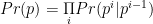
We would  like to recommend playlist of songs.  More generally, we seek to estimate the probability of observing a new, directed sequence , given a training set of a very large set of directed sequences  .  To do this, we define a conditional, probabilistic, vector space model  that retains the local sequence structure of the sample data, and we try to learn the optimal model via regularized maximum-likelihood estimation (MLE) .

Developed by Joachims (and following his notation), we seek to predict a (directed) sequence of states (i.e. an ngram sequence, a playlist of songs, etc. ) from a large collection of states , where .   We model each sequence as a Markov Chain, so that

We embed the sequence into the Latent space, or the d-fold Tensor space  (which is isomorphic to a dimensional Euclidean space )

, such that  

The inference problem is to find  ; it is  solved using a straightforward Stochastic Gradient Descent (SGD) algorithm, restricted to a kind of nearest-neighbor sampling called a Landmark Heuristic

Because we have a Markov Model, we will see that all we need is to write down the local log-Likelihood, defined through the conditional transition probabilities  , and, as usual, some regularization.  Joachims ignores long range interactions and only regularize locally, and I will note some opportunities to address this.

Also, we note that assuming a Markov Model is actually restrictive (Recall our post on Brownian motion and memory effects in chemical physics) .  First, it assumes that to predict the next song, the only songs that matter are the ones we listened to before this song.  Additionally, Markov Models can ignore long-range interdependencies.   A NMF based recommender does not assume this, and they include long-range effects.

Recent work (2013) shows how to parallelize the method on distributed memory architectures, although we will do all of our work on a shared memory architecture. they even provide sample code!

Visualizing the Embedding

For example, a typical embedding is visualized as:

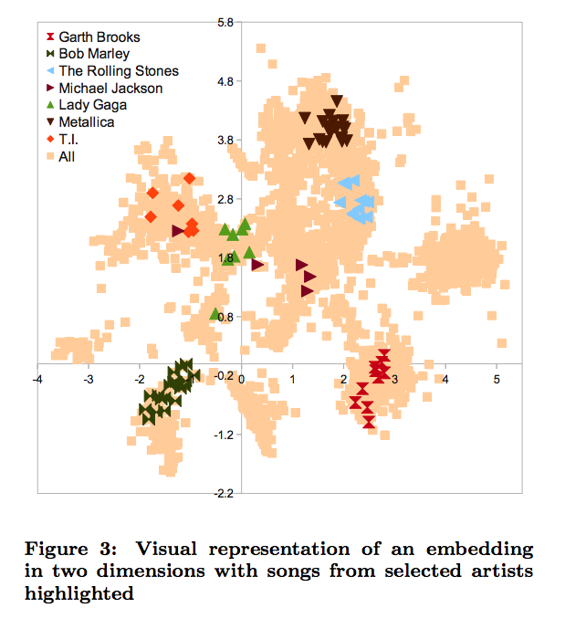
The Online LME Demo provides an interactive view of the embedding.  It also includes simple modifications for adding popularity, user bias, and even semantic tags to the model (not discussed here)

Single and Dual Point Logistic Metric Embeddings

Joachims introduces 2 different models, called the Single Point and Dual Point models.  We  should only care about the Dual Point model, although, curiously, in the published paper (2012), the Dual Point model does not work better than the Single Point model.  So, for now, we describe both. Also, the code contains both models.

By a Metric Embedding, we mean that the conditional probability is is defined with the metric, or distance , in the Latent space where we have embedded our states (songs).

What is the Embedding?

We associate each state  with a vector

Notice Joachims writes  and  to distinguish between vectors associated with elements of a playlist and arbitrary elements of .

In a model for , say, playlists, each vector  it is , initially, just a point  on a -dimensional hypercube.  We then run an inference algorithm which learns the optimal vectors  that minimize the total regularized log-likelihood , as computed over the entire training data, and subject to the specific model chosen.

What is ?

In the Single Point model,  is just the Euclidean distance between   and

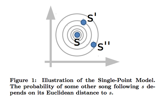
This is just a standard Vector Space model.

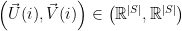
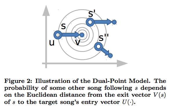
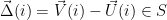
In the Dual Point model, however, we associate 2 points (vectors)  , with each state within a  sequence .  We call these the entry and exit points.

The distance between 2 states the asymmetric divergence

This is like a Vector Field Model, where each state is mapped to a directed vector

.

(In mathematical physics, the embedding is a called a Vector Field or, more generally, a Fiber Bundle ).

The Latent metric is the Euclidean distance between the end point of and the starting point of  within a directed sequence .

We can also construct sequence-independent ()  vectors by simple averaging over a large sample of known sequences (i.e. song playlists).

Model Inference

We want to find

where   is the point partition function, given by

This is just the normalization of the conditional probability (above).   Note that  the  sum is over all possible states , and for numerical performance, we will restrict the sum to nearby states.  

Actually, the final model used is somewhat more complicated because it includes other features to adjust for popularity, user bias, diversity, etc.

Final LME Model

The optimal solution is found by maximizing the  log-Likelihood , subject to regularization to avoid over-training.

in this related post, I explain the partition function and where it comes from.

For the Single Point Model, the objective function is the log-Likelihood plus a standard 2-norm regularizer

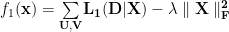
For the Dual Point Model, the objective function includes 2 kinds of regularizers

The first regularizer is

and ensures that the entry and exit vectors don’t get too large.  It is similar to the kind seen in traditional matrix factorization techniques.

The second regularizer ensures the small length sequences, and is similar in spirit to the kind of path regularizers seen  in Minimum Path Basis Pursuit methods (where, ideally, we would seek use an L1-norm for this).  This part is critical because it allows to decompose what looks like a large, messy, non-convex, global optimization problem into a convex sum of local, albeit non-convex , optimization problems:

A Local Manifold Optimization Problem

Here is the real trick of the method

By including  the dual point, local path regularizers ,  we can represent the global log-Liklihood as a sum over local log-Likelihoods, describing regularized transitions from 

We re-write the  objective function (here, Joachims  confuses the notation and includes the regularizer in the log-Likehood, so be careful)

where

• is the collection of states close to (i.e  all nearest neighbors,  observed bigams, etc.),
• is the number of transitions from , and is precomputed from the training data, and
• is the dual point, local log-likelihood term for the transition

• is the global regularizer, but which is trivial to evaluate locally (using SGD)

While the optimization problem is clearly non-convex, this decomposition allows us to ‘glue together’ a convex combination  of locally non-convex but hopefully tractable optimizations, leading to what I call a manifold optimization problem.   ( Indeed, from the point of view of mathematical physics, the dual point embedding model has the flavor of a non-trivial fiber bundle,  and the path constraints act to minimize the curvature between the bundles; in other words, a gauge field theory. )   Usually I don’t trust non-convex methods.  Still,  it is claimed good solutions can be found with 100-200 iterations using standard SGD.  We shall see…

SGD Update Equations

Joachims suggests solving the SGD by iterating through all states (songs) and updating the exit vectors with

and for each , updating the entry vector for each possible transition

where

• is the SGD learning rate, and
• is the number of transitions sampled

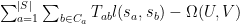
The partials over the regularizers are simple

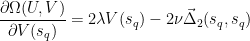
The partial over  is written to  samples all possible exit vectors

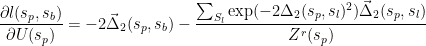
while the partial over is considerably simpler since we only sample the individual transitions (from exit to entry) for each state, yielding

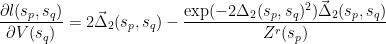
Notice refers to a restricted partition fucntion that only samples states in (i.e nearest neighbors, or what Joachims called the Landmark Heuristic)

Possible Extensions

In a simple Netlfix-style item recommender, we would simply apply some form of matrix factorization (i.e NMF) to   directly, and ignore the sequence structure.  Here, it is noted that we have some flexibility in computing   , and we could both Kernalize and Regularize it before running the inference algorithm.

Next Steps

Now that we have a basic review of the model, it would be fun to make some personalized playlists.  This can be done using the online LME Software. Have fun exploring!

References

See Joachims Website on Playlist Prediction and the references list