Previously we developed some intuition behind the Radial Basis Function / Gaussian Kernel by looking at its Fourier components. We learned that an RBF Kernel is an infinite sum of Laplacians (spatial derivatives) and that, as a Regularizer, it selects out smooth solutions for an ill-posed Inverse problem.
We also learned that in physics, we use the machinery of Kernels to describe the Coherent States. Coherent States are an over-complete, continuously varying, infinite basis of non-orthogonal functions that we constructed from an infinite sum of orthogonal, Quantum Harmonic Oscillator (QHO) basis functions.

We examine the Spectral Properties of the Gaussian Kernel; we will find that the eigenfunctions of the Gaussian Kernel are eigenfunctions of the Quantum Harmonic Oscillator (QHO) .
We will then see how to interpret this correspondence with physics by modeling each data point as a super simple quantum mechanical particle. This part work is based on some semi-recent papers by Shi et. al. As usual, this may take 3-4 blogs.
For now, let’s take a deeper look at the eigenspectra of the Gaussian Kernel. See Fasshauer & McCourt for details. Here I present the basic results, fixing the notation so we can compare the Machine Learning result with the physics.
Modeling with a Gaussian Kernel
When we model data with a vector space, and with a Laplacian or a Kernel, we have a choice to model the individual data points 


When 

Lets consider the one dimensional case
where the functions 

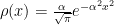

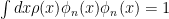
As with our Coherent States, we change the measure rather than change the eigenfunctions. We could, of course, equivalently define

Hermite Polynomials: Generating Functions
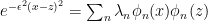
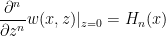
How can we find the eigenfunctions? Note that the RBF function is the Generating Function for the Hermite Polynomials. Let 

We can derive all known properties of the Hermite Polynomials from

In particular, we can solve for various integral relations, although usually we can also look up the relations in a table of integrals (i.e. Gradshteyn and Ryzhik). To derive our result, most papers site equation (39) in the older paper by Zhu et. al. is

although, thanks to the Wikipedia, today we can just look up Mehler’s formula directly

This gives us some insight into the spectrum of the RBF Kernel; we may expect the eigenfunctions to be some scaled Hermite polynomials, under the proper measure. We will need to work though all the messy details. Instead, I will present the central result and some older and newer references. Then take a look at some results from actual calculation
Orthogonal Spectrum of the RBF Kernel: Hermite Polynomials
Here I present some older results; newer relations are found in the 2 papers by Shi et. al.
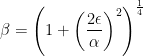
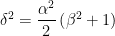
As shown in Fasshauer & McCourt, the eigenvalues 


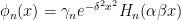

where 
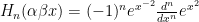
and

With this result, it is possible to apply the traditional spectral techniques, similar to Spectral Clustering, to analyze data sets in machine learning. For example, Shi et. al. use apply RBF basis functions to create probabilistic mixture models to describe their data .
We will look at this work more closely below; let us first lay out the intuition for this approach from known results and approaches in quantum physics and quantum chemical specroscopy.
Quantum Mechanical Harmonic Oscillator:
With a little physics review, a change of variables, and some scaling, we will soon see that the eigenfunctions of the RBF Kernel are, in fact, the same as the stationary states of the Quantum Harmonic Oscillator (QHO).
Of course, the eigenvalues / energy levels are quite different; the RBF eigenvalues approach zero as n increases, whereas the QHO energy levels are evenly spaced.
(Latex is acting up…I’ll get back to writing this up)
Data Spectroscopy: Quantum Mechanical Data Modeling
Imagine if we to consider each data point in $latex\mathbb{R^{n}} $ as some quantum mechanical particle, and suppose we want to compute total probability density of the collection of points. We do this using techniques of Spectroscopy, meaning we will express the Hamiltonian of the system in a primitive basis and diagonalize it. What basis? These are simple, bound particles, so pick the simplest basis possible–Harmonic Oscillators. So each data point is a little QHO, and we seek to model the entire collection. This is the physical intuition behind the Data Spectroscopy
References:
C. E. Rasmussen & C. K. I. Williams, Gaussian Processes for Machine Learning
Huaiyu Zhu, Christopher K. I. Williams, Richard Rohwer & Michal Morciniec, Gaussian Regression and Optimal Finite Dimensional Linear Models
G. E. Fasshauer & M. J. McCourt† Stable Evaluation of Gaussian RBF Interpolants
T. Shi, M. Belkin, and B. Yu, DATA SPECTROSCOPY: EIGENSPACES OF CONVOLUTION OPERATORS AND CLUSTERING
T. Shi, M. Belkin, and B. Yu, Data spectroscopy: learning mixture models using eigenspaces of convolution operators

Very, very interesting your blog. Would you mind continuing your blog on data-spectroscopy?
LikeLike
ill try to get around to it…keep asking
LikeLike
ill try to get to it…been tied up
LikeLike