A lot of my ideas about Machine Learning come from Quantum Mechanical Perturbation Theory. To provide some context, we need to step back and understand that the familiar techniques of Machine Learning, like Spectral Clustering, are, in fact, nearly identical to Quantum Mechanical Spectroscopy. As usual, this will take several blogs.
Here, I give a brief tutorial on the theory of Spectral Clustering and how it is implemented in open source packaages
At some point I will rewrite some of this and add a review of this recent paper Robust and Scalable Graph-Based Semisupervised Learning
Spectral (or Subspace) Clustering
The goal of spectral clustering is to cluster data that is connected but not lnecessarily compact or clustered within convex boundaries

The basic idea:
- project your data into
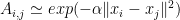
- define an Affinity matrix
, using a Gaussian Kernel
or say just an Adjacency matrix (i.e.
- construct the Graph Laplacian from
- solve an Eigenvalue problem , such as
(or a Generalized Eigenvalue problem
)
- select k eigenvectors
corresponding to the k lowest (or highest) eigenvalues
, to define a k-dimensional subspace
- form clusters in this subspace using, say, k-means


Sounds simple enough. Lets dig into the details a bit to see what works.
Affinities and Similarities
What is an Affinity? It is a metric that determines how close, or Similar, two points our in our space. We have to guess the metric, or we have to learn the metric. For now, we will guess the metric. Notice it is not the standard Euclidean metric. The next simplest thing is, of course, a Gaussian Kernel.
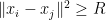
Given 2 data points 


We might provide a hard cut off 

and in some applications, we pre-multiply
( We may also learn the Affinity Matrix from the data. For example, see Learning Spectral Clustering by Bach and Jordan http://www.di.ens.fr/~fbach/nips03_cluster.pdf )
Of course, 


Generally we use the Gaussian Kernel
Here, I want to point out the obvious relation between the Gaussian Kernel

The unnormalized Graph Laplacian is defined as the difference of 2 matrices

where 


When using an Adjacency Matrix, the weights are all 1:
So, apart from the diagonal and some normalization, we see that the Graph Laplacian for an Adjacency Matrix s a low order approximation to the Gaussian Kernel, which is a good approximation when 
In the real world, one usually applies a Gaussian or Heat kernel in order to account for irregularities in the data, as in the SciKit learn package.
Laplacians
There are lots of Laplacians
They all share the Degree matrix

being an old physical chemist, I think of this as a local (nearest neighbor) mean-field average of the Affinity;
We can now define the Laplacian and outline some variations
The main differences are how one normalizes the data and sets the diagonal of 
- Simple Laplacian
- Normalized Laplacian
- Generalized Laplacian
- Relaxed Laplacian
- Ng, Jordan, & Weiss Laplacian
, and where
- and we note the related, smoothed Kernel for Kmeans Kernel Clustering


What are the main differences? Left multiplying by a diagonal matrix is akin to scaling the rows, but right multiplying by a diagonal matrix is akin to scaling the columns. The generalized Laplacian results in a right-stochastic Markov matrix ; the normalized Laplacian does not.
I might have missed some variations since clearly there is a lot of leeway and creativity in defining a Laplacian for clustering. In a future post I will explain how these Graph Laplacians are related to the classical Laplacian from physics. The Von Luxburg review attempts to clean this up, and I may re-write this section based on his review.
The Cluster Eigenspace Problem
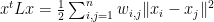
If good clusters can be identified, then the Laplacian 
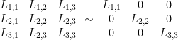
Where 


We also expect that the 3 lowest eigenvalues & eigenvectors 


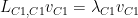
then 

More importantly, this also restricts the eigenvalue spectrum of


Also, to identify k clusters, the eigenvalue spectrum of

Frequently this gap is hard to find, and choosing the optimal k is called “rounding”
I am being a bit sloppy to get the general ideas across. Technically, running Kmeans in the subspace is not exactly the same as identifying each eigenvector with a specific cluster. Indeed, one might imagine using a slightly larger subspace than necessary, and only extracting the k clusters desired. The subtly here is getting choosing the right Affinity ( matrix cutoff R and all), the right size of the subspace, and the right normalization (both of the Laplacian and the eigenvectors themselves, before or after diagonalization) You should refer to the original papers, the reviews, and whatever open source code you are using for very specific details.
Recently (well, kinda, 2008), these ideas have been formalized in L. ROSASCO, M. BELKIN, E. DE VITOA NOTE ON PERTURBATION RESULTS FOR LEARNING, EMPIRICAL OPERATORS
using some perturbation theory and the Resolvent Operators introduced earlier…which gives you an idea of what I like to read just for fun.
[ In the language of Quantum Mechanical Perturbation Theory, we would say that the eigenvectors of the subblocks form a Model Space that approximates the true low lying (or high lying) Eigenspace of
Constraints on Real World Data
Below we depict the block structure of the Affinity matrix for good and poor cases of the Similarity metric

Notice that the good Similarity / Affinity matrix is itself block diagonal when 2 clear clusters can be identified
Open Source Implementations
The Python toolkit Scikit Learn has an implementation of spectral clustering.
Rather than review this, I just want to comment on the 2 examples because neither actually demonstrate where the method is most useful.
The first example is simply to identify 4 overlapping circular clusters. Here, even simple Kmeans would probably be fine because the clusters are compact. They argue the point is to separate the clusters from the background, but, again, this is a simple problem.
The second example is the classic Lena image.

Here, the method does not do much because simple Spectral Clustering can not ‘learn’ from other examples. Here really one wants a supervised or semi-supervised method such as SemiSupervised Learning using Laplacian / Manifold Regularization or even Deep Learning that can identify faces based on a large training sample of many images of many different faces.
The power of Spectral Clustering is to identify non-compact clusters in a single data set (see images above)
Stay tuned
The constraint on the eigenvalue spectrum also suggests, at least to this blogger, Spectral Clustering will only work on fairly uniform datasets–that is, data sets with N uniformly sized clusters. (This is also briefly mentioned by Von Luxburg , where she suggests always using the Generalized Laplacian.) Otherwise, there is no guarantee that the full space and subblock eigenspectrums will line up so nicely.
Some time later, I will take a look at some real world data, look at Andrew Ng’s old argument about matrix perturbation theory, and then explain how to apply matrix perturbation theory to (hopefully) deal the cases of a Poor similarity measure (right side above) .
But first, we take a look at some more modern work by Shi, Belkin, and Yu, called Data Spectroscopy. We will see that Spectral Clustering with an RBF Kernel is, in essence, just like Quantum Mechanical Spectroscopy where the data points are Quantum Mechanical Harmonic Oscillators!
Then we will look at generalizations of Spectral Clustering such as using the Graph Laplacian as a Regularizer for SemiSupervised Manifold Learning.
References
Von Luxburg, A Tutorial on Spectral Clustering, http://www.kyb.mpg.de/fileadmin/user_upload/files/publications/attachments/Luxburg07_tutorial_4488%5B0%5D.pdf
Filippone, Camastra, Masulli, & Rovetta ,A survey of kernel and spectral methods for clustering, http://lagis-vi.univ-lille1.fr/~lm/classpec/publi_classif/A_survey_of_kernel_and_spectral_methods_for_clustering_PR_2008.pdf
Smola and Kondor, Kernels and Regularization on Graphs http://enpub.fulton.asu.edu/cseml/07spring/kenel_graphs.pdf
and one of the more “popular” papers
Ng, Jordan, and Weiss, On Spectral Clustering: Analysis and an Algorithm, http://ai.stanford.edu/~ang/papers/nips01-spectral.pdf

Thanks for the post!
The normalized Laplacian is not the same as the generalized Laplacian. Left multiplying by a diagonal matrix is akin to scaling the rows, but right multiplying by a diagonal matrix is akin to scaling the columns.
The generalized Laplacian results in a right-stochastic Markov matrix (assuming A_{ij} were all non-negative in the first place), but the normalized Laplacian does not.
Also, another cool kernel graph-related kernel is the graph Laplacian kernel:
$$ K = (I + \gamma L) ^ {-1} $$
see: http://enpub.fulton.asu.edu/cseml/07spring/kenel_graphs.pdf
LikeLike
Thanks for the clarification. I did not think anyone ever read this. 🙂 I’ll make the correction
I think what you call the graph Kernel Laplacian is what I call a resolvent operator
https://charlesmartin14.wordpress.com/2012/09/28/kernels-greens-functions-and-resolvent-operators/
LikeLike
“5 . select k eigenvectors \{ v_{i}, i=1, k \} corresponding to the k lowest (or highest) ” .. when should we use lowest or highest eigen vectors
“Ng, Jordan, & Weiss Laplacian L_{NJW}=D^{-1/2}AD^{-1/2}, and where A_{i,i}=0 ” .. but U Von Luxburg 2007 used L instead of A (section 3.2)
LikeLiked by 2 people
its a sign issue and I can’t recall which one. what I would do is just look at a toy problem and select the lowest or highest eigenvector and see how many nodes (zero crossings) its has. the one you want has the fewest nodes. lets look at scikit learn and see what it does–this is implemented there
LikeLike
Charles,
Big fan of your blog. I am curious if you can give a relationship to the work that is being done in persistent homology. To me that approach is a more general approach to solving clustering over non-compact sets of points and has some similar undertones (in the most abstract sense the eigenvalue jump seems reminiscent of barcodes)
LikeLike
yes, it is very similar. indeed, in this video, they explain the relationship between the homology and the eigenspectra: http://videolectures.net/icml08_belkin_dslmm/
i have not personally compared the techniques but i imagine it is possible to apply techniques of data spectroscopy at different levels of scale, thereby obtaining the same kind of graphical results that the Ayasdi guys get using persistant homology. Remember that the homology approach requires defining a similarity metric, and this is equivalent to defining a kernel, so compact or not, one still needs a metric embedding.
Clearly the spectrum depends on the kernel, and most people just use an RBF kernel because it is convenient.What is curious to me is that this spectral approach is equivalent to what is done in quantum field theory, where we represent the field quanta (data points) using quantum mechanical harmonic oscillators, and then solve for the clusters by minimizing an energy functional. On the spectral gap, the case I describe here is very idealized, and I imagine that the common data spectra is could be difficult to partition
LikeLike
Great overview with pointers to unifying different fields.
Subspaces are sparsity inducing transformations in compressed sensing. As you point out, learning the prior from samples is the tricky bit.
Do you know if for image processing, noise rejection in patch-space (non local means) can be augmented with anisotropic local kernels? E.g. use a simple RBF first then re-use the connectivity “local direction” to smooth density better and reinforce that topology clarifying cluster boundary smoothness.
Database normal forms are more strictly block diagonal but I imagine search and inference applications can use such probabilistic structure to execute queries – essentially set algebra. This might become feasible if performed on subsamples viz.Clustering Partially Observed Graphs via Convex Optimization. Ali Jalali, Yudong Chen, Sujay Sanghavi, Huang Xu.
LikeLike
I think that whenever you try to do some kind of local smoothing, you risk over-fitting. One way to treat this is to smooth at different levels of resolution and look for a persistent topology.
LikeLike
i dont know much about it but it sounds interesting
thanks for the link
LikeLike
One tiny comment … Von Luxburg is a she not a he 🙂
LikeLike
thanks…correction made
LikeLike
One comment about
“This is also briefly mentioned by Von Luxburg , where she suggests always using the Generalized Laplacian”.
Von Luxburg tells that “As using Normalized Laplacian also does not have any computational
advantages, we thus advocate for using Generalized Laplacian”, which I find a bit not correct, since normalized Laplacian is a real symmetrical matrix with clear computational advantages, which is not the case for the Generalized Laplacian.
Of course, both matrices have the same eigenvalues, and eigenvectors are just scaled. However, I would use Normalized Laplacian instead of the Generalized one, especially if the computational time is of concern (there are such applications).
LikeLike
Hi,
would this algorithm face Local Minima problem like K-Means, I am new to Data Science, and this looks very promising but I am not sure, It definitely looks better than K-Means, as it handles Non-Convex data but if you were to compare the two algos what Pros and Cons would you notice. How to approach these algorithms, can you please advice.
Regards,
LikeLike
Charles,
While your presentations is indeed quite nice, I would appreciate (and so would others), if there is a follow up. How can one use the Laplacian (lets say, 1, 3 and 5) to perform out-of-sample extension? As I see, 3, 5 solves a different eigenvalue problem, while 1 solves another one. Most implementations/descriptions in literature are of no use as they do not work.
LikeLike
this is not simple in general. see http://papers.nips.cc/paper/4560-semi-supervised-eigenvectors-for-locally-biased-learning.pdf
LikeLike
Charles,
That paper is indeed quite useful. I will read it carefully. The papers that I was looking at are the following:
Click to access data_2009.pdf
Essentially, LE (as per your notation, 1, 2 or 3) has a property that is described in Sec 3.2.1 of the paper, wherein the mapping of the new sample is a weighted average of the existing mapping (Eq. 9) of the paper.
I don’t think they are using LE4 or LE5.
Now, if we introduce the notion of class labels
Click to access A%20supervised%20non-linear%20dimensionality%20reduction%20approach%20for%20manifold%20learning.pdf
then,
I would presume that the mapping obtained from the previous paper should also hold.
What I am seeing is the following:
a.) I am able to see good class separation when I use Dornaika’s clas-label based LE
b.) However, when I use the mapping generated by a.) and apply Eq 9 from the first paper, I cannot see any good data separation. So, what could I be doing wrong? Am I even thinking correctly here?
LikeLike
and my earlier blog posts on semi superrvised clustering
LikeLike
I think Ref # 11 in the above paper is quite useful
LikeLike
Hi,
my question is about the affinity matrix; can we use any measure of similarity that we can imagine to define it? is there some constraint about its definition?
Thank you
LikeLike
It’s unclear . Usually these methods only work for data that is fairly uniform in distribution in the Hilbert space the matrix acts in
LikeLike
Reblogged this on Braveheart.
LikeLike
what i understand from this reading, is that i don’t need to apply pca before clustering if i’m using spectral clustering, am i right?
for example, if i have a set of points of 10 dimensions, and i want to find the clusters, but i don’t know which dimensions are the most relevant, i don’t need to choose the dimensions, as spectral clustering does that as part of the process?
if spectral clustering is what i need for this example, what preprocessing do i need to do (normalization, determine the number of dimensions, determine the number of clusters)?
should i look for another tool (which one)?
LikeLike
You need more than 10 points to apply clustering effectively.
LikeLike
You just need to form the laplacian usually normalized
LikeLike